Transformation of Several Data Frame Objects/Variables into one Tidy (Long Table) Form
Source:R/transform_dfs_2tidyDF.R
transform_dfs_2tidyDF.RdTaking several data frame objects from the (local/Global) R environment and transforming them into
one with the long table/tidy form. This is especially handy
if a quick comparison of similar plots/EPR spectra in one graph panel is required. Difference between
the readEPR_Exp_Specs_multif and the actual function lies in the object input/origin.
While the readEPR_Exp_Specs_multif takes the original files/data, coming from spectrometer,
the transform_dfs_2tidyDF collects temporary processed/stored data frame objects/variables
created meanwhile in the R environment.
Arguments
- ...
Data frame object names (separated by comma
,) to be transformed into long table/tidy form in order to quickly compare plots/EPR spectra in one graph panel (see alsoExamples). The number of data frame vobjects is not limited, however for the series of \(\geq 10-12\) objects/spectra, the graph may look cluttered, depending on complexity of EPR spectra.- df.names
Character string vector of labels (in the form of e.g.
c("Spectr_01","Spectr_02")orc("283 K","273 K","263 K")), describing the individual data frames/plots in the returned tidy/long table and corresponding to series of plots/spectra (be aware of the data frames order).- which.coly.norm
Character string, pointing to name of the column (in all data frame objects) to be normalized, by the
norm.vecvector. This column actually corresponds to quantity/variable presented on graph as y-axis. Default:which.coly.norm = "dIepr_over_dB"(that is the derivative intensity in CW EPR spectra).- norm.vec
Numeric vector, consisting of (division) normalization constants (see also the
which.coly.normargument) for each of the data frame objects defined by the ellipsis...argument. Default:norm.vec = rep(1, times = length(df.names)), i.e. all normalization constants equal to1. If needed, the vector may be redefined (please, be aware of the data frames order).- var2nd.series
Character string, pointing to name of the second variable which is "common denominator" for the series of
df.namesvector elements likevar2nd.series = "Temperature"orvar2nd.series = "Spectrum"(default).
Value
Tidy (long form) data frame/table object, carrying all the individual inputs, defined by the ...
argument and ready for the overlay/offset plot to compare the data in desired series.
Note
In order to compare \(g_{\text{iso}}\)-values of different EPR spectra, prior to own transformation
check that all data frame objects contain g_Val(ue) variable/column. If this is not case,
the user may create those columns by the eval_gFactor function.
Examples
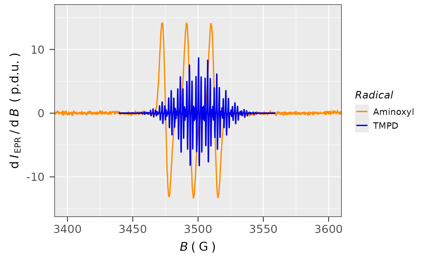
## compare TMPD*+ EPR spectrum with that of aminoxyl,
## first, define the path and variable for TMPD*+ data
tmpd.data.path <-
load_data_example(file = "TMPD_specelchem_accu_b.asc")
tmpd.data.df <-
readEPR_Exp_Specs(
tmpd.data.path,
col.names = c("B_G","dIepr_over_dB"),
qValue = 3500,
origin = "winepr"
)
#
## preview
head(tmpd.data.df)
#> B_G dIepr_over_dB B_mT
#> 1 3439.1699 -56.047361607 343.91699
#> 2 3439.2200 -30.506506697 343.92200
#> 3 3439.2700 -38.522218750 343.92700
#> 4 3439.3201 0.039208426 343.93201
#> 5 3439.3701 -92.620223214 343.93701
#> 6 3439.4199 -71.915075893 343.94199
#
## second, do the same for the aminoxyl data
aminoxyl.data.path <-
load_data_example(file = "Aminoxyl_radical_a.txt")
aminoxyl.data.df <-
readEPR_Exp_Specs(
aminoxyl.data.path,
qValue = 2100
)
#
## preview
aminoxyl.data.df %>% head()
#> index B_G dIepr_over_dB B_mT
#> 1 1 3332.7000 -1.7738564e-06 333.27000
#> 2 2 3332.9005 1.2209461e-07 333.29005
#> 3 3 3333.1009 -1.8403788e-07 333.31009
#> 4 4 3333.3014 -7.1641412e-08 333.33014
#> 5 5 3333.5019 -1.7361444e-06 333.35019
#> 6 6 3333.7023 -5.1531169e-07 333.37023
#
## ...and the own transformation
spectra.data.tidy.df <-
transform_dfs_2tidyDF(
tmpd.data.df,
aminoxyl.data.df,
df.names = c("TMPD","Aminoxyl"),
norm.vec = c(5e+3,1e-5),
var2nd.series = "Radical"
)
#
## preview
head(spectra.data.tidy.df)
#> Radical B_G dIepr_over_dB B_mT
#> 1 TMPD 3439.1699 -1.1209472e-02 343.91699
#> 2 TMPD 3439.2200 -6.1013013e-03 343.92200
#> 3 TMPD 3439.2700 -7.7044437e-03 343.92700
#> 4 TMPD 3439.3201 7.8416853e-06 343.93201
#> 5 TMPD 3439.3701 -1.8524045e-02 343.93701
#> 6 TMPD 3439.4199 -1.4383015e-02 343.94199
#
## plotting both EPR spectra together
plot_EPR_Specs(
data.spectra = spectra.data.tidy.df,
x = "B_G",
x.unit = "G",
var2nd.series = "Radical",
var2nd.series.slct.by = 1,
xlim = c(3400,3600),
line.colors = c("darkorange","blue2"),
legend.title = "Radical"
)
 #
## ...and the interactive preview (B in mT)
plot_EPR_Specs2D_interact(
data.spectra = spectra.data.tidy.df,
line.colors = c("darkorange","blue2"),
var2nd.series = "Radical",
legend.title = "Radical"
)
#
## ...and the interactive preview (B in mT)
plot_EPR_Specs2D_interact(
data.spectra = spectra.data.tidy.df,
line.colors = c("darkorange","blue2"),
var2nd.series = "Radical",
legend.title = "Radical"
)