Overview 
The key objective of this open source ![]() package is to bring handy functions corresponding to “everyday” data processing/analysis in the EPR (Electron Paramagnetic Resonance) spectroscopy mainly for chemists. Similar
package is to bring handy functions corresponding to “everyday” data processing/analysis in the EPR (Electron Paramagnetic Resonance) spectroscopy mainly for chemists. Similar ![]() tools like cwepr and the related projetcs have been developed, so far. The eprscope, as the first complex
tools like cwepr and the related projetcs have been developed, so far. The eprscope, as the first complex ![]() package 📦 for EPR, doesn’t want to replace the latter nor the excellent and standard EPR simulation/processing EasySpin Toolbox for MATLAB and its additional frameworks like SpecProFi or CW EPR Scripts by Emilien Etienne. Rather, it may be considered like a complementary 📦 or toolbox with practical functions which have to be otherwise performed by several proprietary tools. For instance, like acquisition/processing software, supplied by the EPR spectrometer manufacturers (see e.g. Xenon/WinEPR) as well as several other software platforms like the MS Office and/or Orgin/SigmaPlot/Igor which are often applied in the EPR processing/analysis workflow. Therefore, the eprscope tries to reduce such many steps/programs. In order to achieve the goal it uses superior power of the open source
package 📦 for EPR, doesn’t want to replace the latter nor the excellent and standard EPR simulation/processing EasySpin Toolbox for MATLAB and its additional frameworks like SpecProFi or CW EPR Scripts by Emilien Etienne. Rather, it may be considered like a complementary 📦 or toolbox with practical functions which have to be otherwise performed by several proprietary tools. For instance, like acquisition/processing software, supplied by the EPR spectrometer manufacturers (see e.g. Xenon/WinEPR) as well as several other software platforms like the MS Office and/or Orgin/SigmaPlot/Igor which are often applied in the EPR processing/analysis workflow. Therefore, the eprscope tries to reduce such many steps/programs. In order to achieve the goal it uses superior power of the open source ![]() ecosystem that combines data processing, analysis and great scientific visualizations together with the extensive publishing capabilities by Rmarkdown and Quarto. Everything at one place (see the RStudio IDE or Positron) without the need to switch between or employ any other additional software.
ecosystem that combines data processing, analysis and great scientific visualizations together with the extensive publishing capabilities by Rmarkdown and Quarto. Everything at one place (see the RStudio IDE or Positron) without the need to switch between or employ any other additional software.
Installation
Prior to own eprscope 📦 installation a minimal system setup is required and summarized into the following steps:
Installation of JDK Development Kit where the corresponding package, suitable for your operating system, can be downloaded from the official Oracle website (this is needed in order to properly run the
draw_molecule_by_rcdk()function). A second option would be the installation of the latest GPL-licensed OpenJDK package. WINDOWS users may follow instructions at the official site of British Columbia Institute of Technology. On macOS, this package is available via the Homebrew repository (see below) bybrew install openjdkand finally, by verifying the installation:java –version. Linux (ubuntu) users are advised to check out the repositories (+ update, if needed):sudo apt update. Then search for theopenjdkby the following command:apt search openjdk(it should return list with the newest/stable version likeopenjdk-XX-jdk, “XX” stands for the highest number), and finally install it bysudo apt install openjdk-XX-jdk -y. After successful installation one may check the version (java -version) .Please, follow the instructions for the the R installation procedure. Linux and macOS users may also update where the
 expects to find various Java files by
 sudo R CMD javareconf(in terminal, not in the R console !), afterwards. If one gets an error aboutjni.hnot being found, then try:sudo R CMD javareconf JAVA_HOME=/usr/lib/jvm/java-XX-openjdk-amd64/(find your exact path for the Java files).Download and install RStudio IDE (Integrated Development Environment). Alternatively, one may also try the corresponding cloud version without the need for an
 installation either available at Posit Cloud or at CoCalc (Collaborative Calculation and Data Science). Any other
  compatible environment like VS Code or Positron may be installed as well.
Download and install the latest release of Rtools (WINDOWS only) or on macOS/Linux follow the instructions to install CMake. Alternatively, on macOS, CMake can be set up via the Homebrew repository (see also https://formulae.brew.sh/formula/cmake#default). This step is required to use the nloptr 📦 for the fitting of isotropic EPR spectra.
-
In the
 Console (lower left panel within the RStudio IDE) run the following code in order to install essential
  packages for data science with all their dependencies ➨
# run code in the R console
#
# after the initial R environment setup it's always
# good to install essential collection of packages for data science
if (!require(pak)) {install.packages("pak")}
pak::pkg_install("tidyverse",dependencies = TRUE)
# ...+ additional required packages with dependencies
pak::pkg_install(
  c("bookdown","kableExtra","tinytable",
    "corrplot","animation","openxlsx","knitr",
    "shinythemes","numDeriv","htmlwidgets",
    "esquisse","nlstools","webshot2"),
  dependencies = TRUE
)
There are two main options how to install the eprscope 📦 via the ![]() Console ➨
Console ➨
# from the GitHub repository:
if (!require(pak)) {install.packages("pak")}
pak::pkg_install("jatanRT/eprscope")
or
# from the R-Universe (https://r-universe.dev/search)
# and CRAN (https://cran.r-project.org/) repositories:
install.packages(
  "eprscope",
  repos = c(
    "https://jatanrt.r-universe.dev",
    "https://cloud.r-project.org"
  )
)
If one wants to install the entire 📦 including all the documentation vignettes/articles ➨
# alternatively, install package together with all the vignettes/articles:
if (!require(devtools)) {install.packages("devtools")}
devtools::install_github("jatanRT/eprscope",build_vignettes = TRUE)
Additionally, the open-source scientific and technical publishing system Quarto together with the Pandoc, a document converter system, may be required for sharing the results coming from eprscope in desired formats like pdf , html , docx , pptx or tex (details may be found in the create_qmdReport_proj() documentation).
Note: On modern Windows systems (10/11), all the pre- and post-installation software packages (OpenJDK, Quarto, Pandoc, LaTeX/Typst and CMake or Rtools) can be easily managed either by Winget or by the Chocolatey systems.
Updates
To update the eprscope 📦, just run the following code (the same as for the installation) in the ![]() console ➨
console ➨
pak::pkg_install("jatanRT/eprscope",upgrade = TRUE)
#
# update package together with vignettes/articles:
# devtools::install_github("jatanRT/eprscope",build_vignettes = TRUE)
Usage
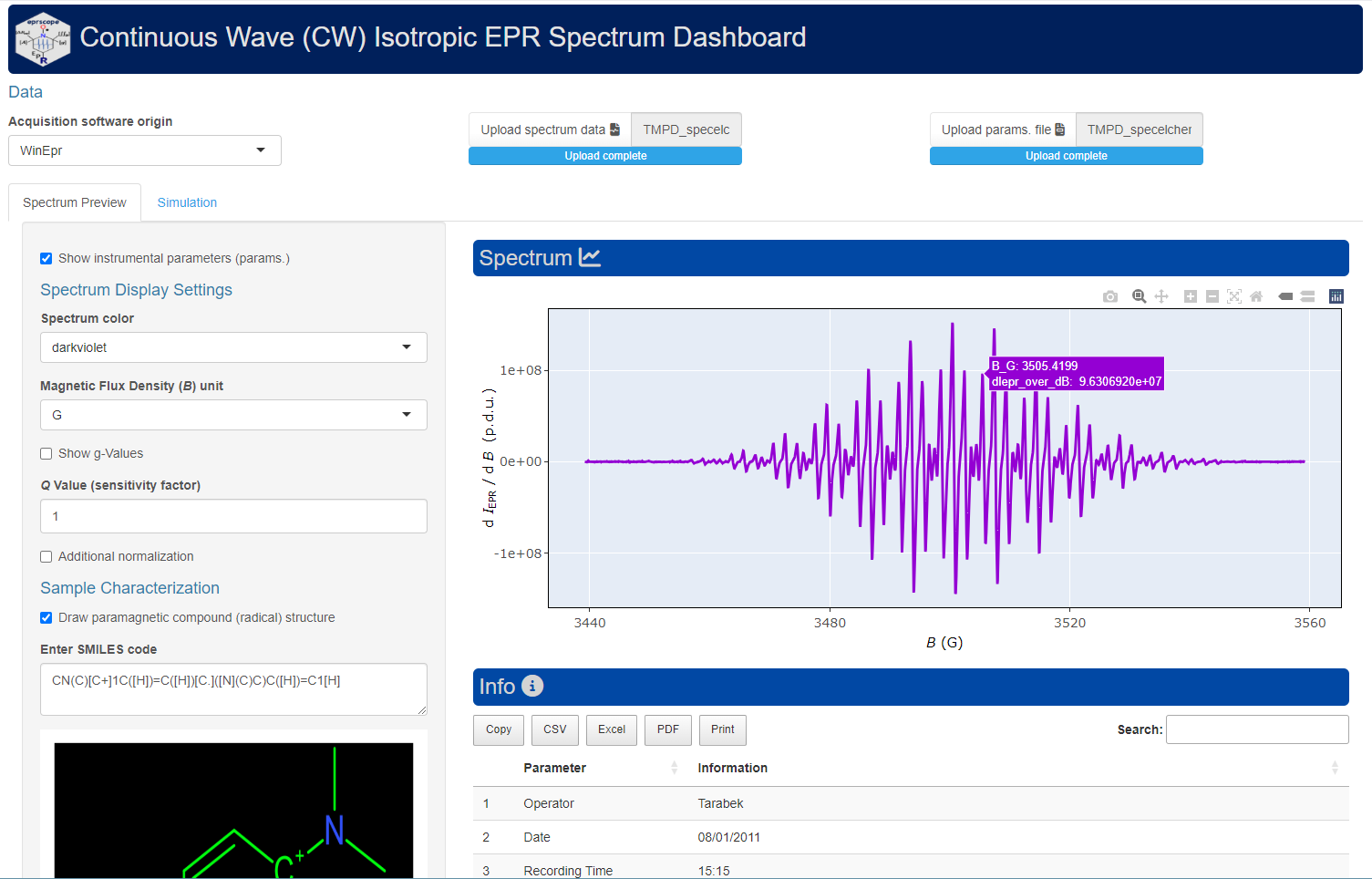
In this section, couple of examples are shown in order to briefly demonstrate the package functionality. More detailed description can be found within the articles/vignettes or in documentation of functions (see Package index/Reference).
Reading Files with Instrumental Parameters
# loading the package/library
library(eprscope)
#
# loading the built-in example file => "TMPD_specelchem_accu_b.par"
tmpd.params.file <-
  load_data_example(file = "TMPD_specelchem_accu_b.par")
#
# parameters into interactive table (data frame)
tmpd.params.dt <-
  readEPR_params_tabs(
    path_to_dsc_par = tmpd.params.file,
    origin = "winepr",
    interact = "params"
  )
#
# table preview
tmpd.params.dt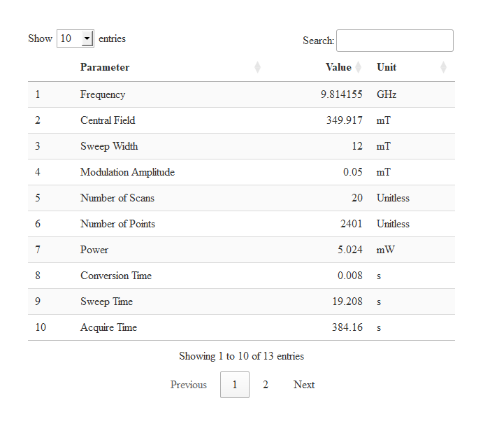
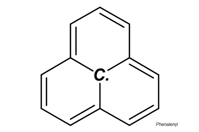
Depict Molecular Structures
# Phenalenyl (Perinaphthenyl or PNT) radical by `SMILES` code:
# "C1([C.]23)=CC=CC2=CC=CC3=CC=C1"
draw_molecule_by_rcdk(
  molecule = "C1([C.]23)=CC=CC2=CC=CC3=CC=C1",
  mol.label = "Phenalenyl",
  mol.label.color = "black",
  mol.label.xy.posit = c(8.8, 1.2)
)
Simulation of Isotropic EPR Spectra
# simulation of the phenalenyl (perinaphthenyl or PNT) radical,
# see also https://pubs.rsc.org/en/content/articlelanding/2006/CS/b500509b,
# the additional experimental/instrumental parameters are not shown,
# they possess their default values => see corresponding documentation
# of the `eval_sim_EPR_iso()` function.
simulation.iso <-
  eval_sim_EPR_iso(
    g.iso = 2.0027,
    B.unit = "G",
    nuclear.system = list(
      list("1H", 3, 5.09), # 3 x A(1H) = 5.09 MHz
      list("1H", 6, 17.67) # 6 x A(1H) = 17.67 MHz
    ),
    lineGL.DeltaB = list(0.24, NULL) # linewidth in G
  )
#
# simulated spectrum preview, in the region from 3470 G to 3522 G
simulation.iso$plot +
  ggplot2::coord_cartesian(xlim = c(3470, 3522))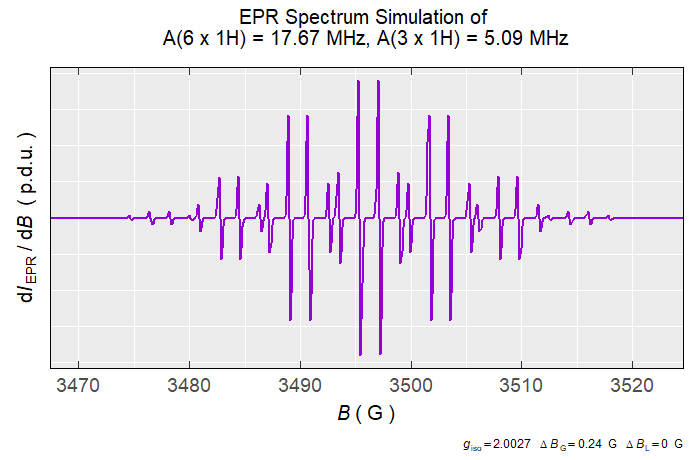
Interactive R Shiny Application to Visualize and Simulate CW Isotropic EPR Spectra
# just run the following command in R console
plot_eval_ExpSim_app()
Radical Kinetic Model Fitted onto the Experimental Data
# decay of a triarylamine radical cation right after
# its generation by electrochemical potentiostatic oxidation
# in TBAPF6/CH3CN, double integrals (Areas) vs time were
# obtained by data pre-processing within the continuous
# wave (CW) EPR spectrometer acquisition/processing software.
#
# loading the built-in example file with the instrumental parameters
triarylamine_rc_decay_dsc <-
  load_data_example(file = "Triarylamine_radCat_decay_a.DSC")
#
# loading the built-in example file with "Area" vs "time" data frame
triarylamine_rc_decay_txt <-
  load_data_example(file = "Triarylamine_radCat_decay_a.txt")
triarylamine_rc_decay_data <-
  readEPR_Exp_Specs(
    path_to_file = triarylamine_rc_decay_txt,
    header = TRUE,
    fill = TRUE,
    select = c(3, 7),
    col.names = c("time_s", "Area"),
    x.unit = "s",
    x.id = 1,
    Intensity.id = 2,
    qValue = 1700,
    data.structure = "others"
  ) %>% na.omit()
#
# fitting the experimental decay by 2R --> B kinetic model
# with "k1" rate constant and the corresponding partial
# rection order "alpha". "qvar0R" refers to the initial
# "quantitative variable" (such as concentration, double integral
# or number of radicals) of the triarylamine radical cation "R",
# for a quick evaluation or comparison with other kinetic data
# "qvarR" corresponds to "Area" (double integral in p.d.u. units)
# and therefore the unit => [k1] = (p.d.u.)^{-1} * s^{-1}
# where the p.d.u. stands for "procedure defined unit"
triarylamine_rc_decay_model <-
  eval_kinR_EPR_modelFit(
    data.qt.expr = triarylamine_rc_decay_data,
    model.react = "(r=2)R --> [k1] B",
    qvarR = "Area",
    elementary.react = FALSE,
    params.guess = c(
      qvar0R = 0.019,
      k1 = 0.04,
      alpha = 1.9
    ),
    time.correct = TRUE,
    path_to_dsc_par = triarylamine_rc_decay_dsc,
    origin = "xenon"
  )
#
# graph preview
triarylamine_rc_decay_model$plot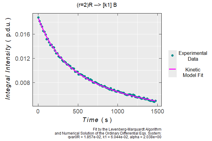
#
# data frame/table, showing the obtained kinetic parameters
# (and their basic statistical measures) by the non-linear
# fit and numeric solution of the Ordinary Differential Equations
triarylamine_rc_decay_model$df.coeffs
#>           Estimate    Std. Error    t value       Pr(>|t|)
#> qvar0R 0.018570037 5.7203136e-05 324.633198 4.3809413e-149
#> k1     0.060438055 5.4514583e-03  11.086585  6.1614969e-19
#> alpha  2.038206072 1.9676205e-02 103.587358 3.9216714e-101
#
# graphical representation of the correlation matrix,
# corresponding to kinetic model fit
triarylamine_rc_decay_model$cor.df %>%
  corrplot::corrplot(addCoef.col = "#c2c2c2")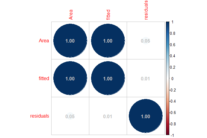
Help, Questions and Contribution
There are several ways how to get help. If the users are already familiar with the R statistical language please, follow either the individual package function documentations or the corresponding articles/vignettes. These might be also considered as a kind of EPR spectroscopy and ![]() knowledge resources. In case you are completely new to R, there are couple of great tutorials (you may also consult the “First Steps with R Language” vignette/article) enabling a quite straightforward diving into
knowledge resources. In case you are completely new to R, there are couple of great tutorials (you may also consult the “First Steps with R Language” vignette/article) enabling a quite straightforward diving into ![]() . Please, refer to e.g.
. Please, refer to e.g.
R Packages and Related Links for Optimization and Mathematical Programming
Reproducible Research in R and Guides for the R-Cubed Courses
Quarto - An Open Source Scientific and Technical Publishing System
-
YouTube Video Tutorials ➨
Even though the EPR spectroscopy is a quite complex field there are some introductory on-line materials which may help to start with this special magnetic resonance method ➨
Any additional questions, comments, remarks or issues can be addressed through several discussion channels like 📧 e-mail jantar40@protonmail.com or github ![]() issues on the github source page (see the contributing guide). In the future, there will be also a specialized Discord community channel to discuss the eprscope related topics. If somebody is able and interested in the package development, please refer to contributing guide.
issues on the github source page (see the contributing guide). In the future, there will be also a specialized Discord community channel to discuss the eprscope related topics. If somebody is able and interested in the package development, please refer to contributing guide.
Acknowledgements
I would like to express a deep gratitude to my colleagues from the NMR Spectroscopy Group of the Institute of Organic Chemistry and Biochemistry especially, Dr. Radek Pohl , Dr. Ondřej Socha
and Dr. Martin Dračínský
. Without the fruitful environment within the NMR Spectroscopy team it wouldn’t be possible to develop such a project like this. Also, I’d like to give a special thanks to my brother Dr. Peter Tarábek
for his valuable comments and remarks.
