EPR spectra often display hyperfine structure, where the spectral lines split into several other ones,
as a consequence of the electron-nuclear interaction with nuclei close to the paramagnetic center.
Sometimes, such splitting can be complicated and requires simulations, i.e. computational "synthesis"
of spectral structure based on quantum chemistry as well as on mathematical description of spectral lineshapes
(see also References). The actual function helps to analyze the hyperfine structure (HFS)
of the isotropic EPR spectra by simulations. For such purpose, properties like nuclear \(g\)-value,
spin quantum number as well as natural abundance of the isotopes, related to interacting nuclei,
must be known and are collected from the isotopes_ds. EPR spectra can be simulated
for the derivative as well as for the integrated line forms (see the argument lineSpec.form).
Usage
eval_sim_EPR_iso(
  g.iso = 2.00232,
  instrum.params = c(Bcf = 3500, Bsw = 200, Npoints = 2048, mwGHz = 9.8),
  path_to_dsc_par = NULL,
  origin = NULL,
  B.unit = "G",
  nuclear.system = NULL,
  natur.abund = TRUE,
  lineSpecs.form = "derivative",
  lineGL.DeltaB = list(1, NULL),
  lineG.content = 1,
  Intensity.sim = "dIeprSim_over_dB",
  plot.sim.interact = FALSE
)
Arguments
- g.iso
Numeric value, guess of the isotropic \(g\)-factor. It may also possess a
NULLvalue if the \(g\) corresponding to "central field" is equal tog.iso. Default:g.iso = 2.00232(the approximate \(g\) of the free electron).- instrum.params
Named numeric vector, containing instrumental parameters required for the simulation =>
Bcf"central field" (magnetic flux density, \(B_{\text{CF}}\)) Bsw"sweep width" (magnetic flux density recording region, \(B_{\text{SW}}\)) Npointsnumber of spectral points (corresponding to resolution) within the "sweep width" mwGHzapplied microwave frequency in GHzto record the continuous wave (CW) EPR spectrumDefault values are chosen to cover the EPR spectra of common organic radicals. If
instrum.params = NULLthen parameters must be provided by thepath_to_dsc_paras well as byoriginarguments.- path_to_dsc_par
Character string, path (can be also acquired by the
file.path) to.DSC/.dscor.par(depending on the OS, seeoriginargument)textfiles including all instrumental parameters from the EPR machine. Default:path_to_dsc_par = NULLin case if theinstrum.paramsis already defined. IF theinstrum.params = NULLthen BOTH thepath_to_dsc_parAS WELL AS theoriginMUST BE DEFINED !- origin
Character string, corresponding to software which was used to obtain the EPR spectra on spectrometers, because the files are slightly different, whether they were recorded by the "WinEpr" (
origin = "winepr") or by the "Xenon". Default:origin = NULLin case no file is used to extract the parameters (i.e. exactly ifpath_to_dsc_par = NULL).- B.unit
Character string, pointing to unit of magnetic flux density which is to be presented on \(B\)-axis of the EPR spectrum, like
"G"(Gauss),"mT"(millitesla) or"T"(tesla), default:B.unit = "G". THE UNIT MUST BE SHARED ACROSS ALL RELEVANT B-ARGUMENTS likecfandswwithin theinstrum.paramsAS WELL AS within THOSE INlineGL.DeltaB!- nuclear.system
List, containing the information about groups of equivalent nuclei interacting with the unpaired electron like
nuclear.system = list("14N",1,45). This corresponds to one group of "14N" interacting nuclei where the second number denotes the number of nuclei within the group and the third number is the guess of the hyperfine coupling constant in MHz. Therefore, in summary it refers to \(A(1\times ^{14}\text{N}) = 45~\text{MHz}\). If more complex interaction is considered, e.g. \(A(3\times ^{1}\text{H}) = 5.06~\text{MHz} + A(6\times ^{1}\text{H}) = 17.64~\text{MHz}\), such system must be defined by nested lists likenuclear.system = list(list("1H",3,5.06),list("1H",6,17.64)). The number oflistsis not limited and therefore, any number of equivalent nuclei groups can be used to simulate the EPR spectra. Default:nuclear.system = NULLin case if no interaction with the unpaired electron surrounding nuclei is considered and only single line EPR spectrum is expected.- natur.abund
Logical, whether the natural abundance of the interacting nuclei is taken into the calculation of intensity pattern of the simulated EPR spectrum. Default:
natur.abund = TRUE. For a single-line EPR spectrum without hyperfine splitting(HFS) it is automatically switched tonatur.abund = FALSE.- lineSpecs.form
Character string, describing either
"derivative"(default) or"integrated"(i.e."absorption"which can be used as well) line form of the analyzed EPR spectrum/data.- lineGL.DeltaB
List of two values referred to as Gaussian (G) and Lorentzian (L) spectral line-forms, respectively. For the "pure" Gaussian only the first value is numeric and the second one is
NULL=> e.g.lineGL.DeltaB = list(1,NULL)(default). For the "pure" Lorentzian the opposite expression must be used => e.g.lineGL.DeltaB = list(NULL,0.5). If the linear combination of both line forms is taken into account (seelineG.content), that is so called pseudo-Voigt, then both values are numeric (e.g.lineGL.DeltaB = list(0.5,0.5)) and are related to Gaussian and Lorentzian forms, respectively. TheDeltaBcorresponds either to \(\Delta B_{\text{pp}}\) (iflineSpecs.form = "derivative") or to \(FWHM\) (iflineSpecs.form = "integrated"or iflineSpecs.form = "absorption"). The unit of values must coincide with those used ininstrum.paramsas well as withB.unit.- lineG.content
Numeric value between
0and1referring to content of Gaussian line form. IflineG.content = 1(default) it corresponds to "pure" Gaussian line form and iflineG.content = 0it corresponds to Lorentzian one. The value from (0,1) (e.g.lineG.content = 0.5) represents the linear combination (for the example above with the coefficients 0.5 and 0.5) of both line forms ➨ so called pseudo-Voigt.- Intensity.sim
Character string, pointing to column of simulated EPR intensity within the related output data frame. Default:
Intensity.sim = "dIeprSim_over_dB".- plot.sim.interact
Logical, whether to display the simulated spectrum by interactive
plotlygraph (see alsoplot_EPR_Specs2D_interact). Ifplot.sim.interact = FALSE(dafault), then the output contains the data frame as well asggplot2based plot of the simulated EPR spectrum within a list.
Value
If plot.sim.interact = TRUE, function returns an interactive plot object with the simulated EPR spectrum.
Otherwise (if plot.sim.interact = FALSE), the output is represented by the list with the following
elements:
- plot
ggplot2static object showing the simulated EPR spectrum.- df
Data frame/table object related to the simulated spectrum.
Details
Theoretical predictions or computations of a spectrum (and its comparison with the experiment) represent
an important step in the analysis of EPR spectra. However, such step requires an iterative process with modelling
the above-described electron-nuclear system followed by a numerical simulations of EPR spectra
to match the experimental ones (see also eval_sim_EPR_isoFit). Commonly, quantum chemical calculations
(usually DFT, see also vignette("functionality") are involved in this process.
EPR simulations in the isotropic regime assume that the molecules tumble/move extremely fast causing a total averaging
of any anisotropic properties out. An EPR spectrum corresponding to the latter consists of a series of symmetric
lines with equal widths. In such case the spectrum is characterized by the isotropic HF coupling/splitting
constants \(A_{\text{iso}}/a_{\text{iso}}\) (see also the nuclear.system argument) as well as
by the above-mentioned linewidth. Many organic radicals exhibit such EPR spectra at room temperature
and in solutions of low viscosities (Gerson F, Huber W (2003), see References).
In the first step the \(B\)-region (magnetic flux density) and the resolution is defined
by the instrum.params argument or can be directly acquired from the parameter file, using
the path_to_dsc_par argument. Position of the spectrum (within the desired \(B\)-region)
as well as those of HFS-lines are evaluated by the resonance condition (see also the eval_gFactor)
and by the Breit-Rabi analytical expression for energy levels of the interacting nuclei.
The related \(B\)s are computed by the fixed-point iterations,
because the corresponding \(g\)-value for each of the HFS-lines is not known (Weil JA (1971)
and Stoll A, Schweiger A (2006)). The shape of spectral lines are calculated by the analytical formula
of linear combination of the Gaussian and the Lorentzian line-shapes (also referred to as pseudo-Voigt,
Weil JA, Bolton JR (2007) and Stoll S (2024)). The linear coefficients
are defined by the lineG.content argument, actually, corresponding to Gaussian line content (the Lorentzian one
is computed as 1-lineG.content, accordingly). The linewidth, from that linear combination,
is specified individually for the Gaussian and the Lorentzian (please, refer to the lineGL.DeltaB argument).
The multiplicities (relative intensity ratios) are computed by the binomial/multinomial coefficients
taking into account the spin quantum numbers of the interacting nuclei, in each of the equivalent groups (please, also
refer to the plot_eval_EPRtheo_mltiplet), as well as their natural abundance (if natur.abund = TRUE).
References
Weil JA, Bolton JR (2007). Electron paramagnetic resonance: elementary theory and practical applications, 2nd edition. John Wiley and Sons. ISBN 978-0-471-75496-1, https://onlinelibrary.wiley.com/doi/book/10.1002/0470084987.
Weil JA (1971). “The Analysis of Large Hyperfine Splitting in Paramagnetic Resonance Spectroscopy.” J. Magn. Reson. (1969), 4(3), 394–399, https://doi.org/10.1016/0022-2364(71)90049-7.
Stoll S, Schweiger A (2006). “EasySpin, A Comprehensive Software Package for Spectral Simulation and Analysis in EPR.” J. Magn. Reson., 178(1), 42–55, https://doi.org/10.1016/j.jmr.2005.08.013.
Stoll S (2024). “EasySpin Documentation - Line Shapes.”, https://easyspin.org/easyspin/documentation/lineshapes.html.
Gerson F, Huber W (2003). Electron Spin Resonance Spectroscopy of Organic Radicals, Biotechnology Series, Wiley-VCH, ISBN 978-3-527-30275-8, https://books.google.cz/books?id=SEPeNjG3IvYC.
Examples
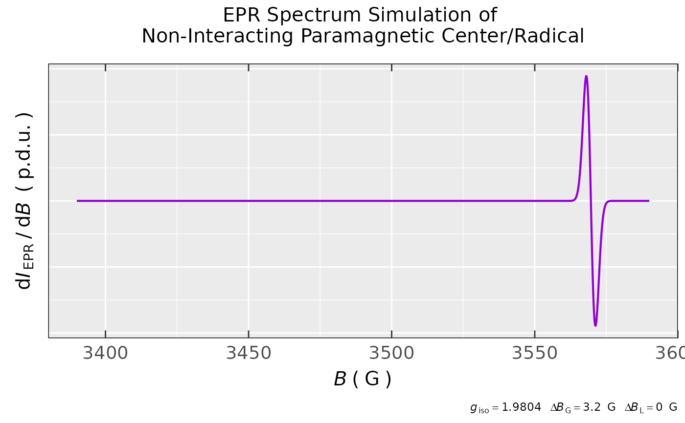
## simulation of simple EPR spectrum (without hyperfine
## structure) with g(iso) = 1.9804 and the linewidth
## ∆Bpp = 3.2 G, only Gaussian lineform is considered:
sim.simple.a <-
eval_sim_EPR_iso(g.iso = 1.9804,
instrum.params = c(Bcf = 3490,
Bsw = 200,
Npoints = 1600,
mwGHz = 9.8943),
lineGL.DeltaB = list(3.2,NULL)
)
## simulation preview:
sim.simple.a$plot
 #
## check the g_{iso}-value
## of the previous spectrum
eval_gFactor_Spec(
sim.simple.a$df,
nu.GHz = 9.8943,
Intensity = "dIeprSim_over_dB",
B = "Bsim_G"
)
#> [1] 1.9804
#
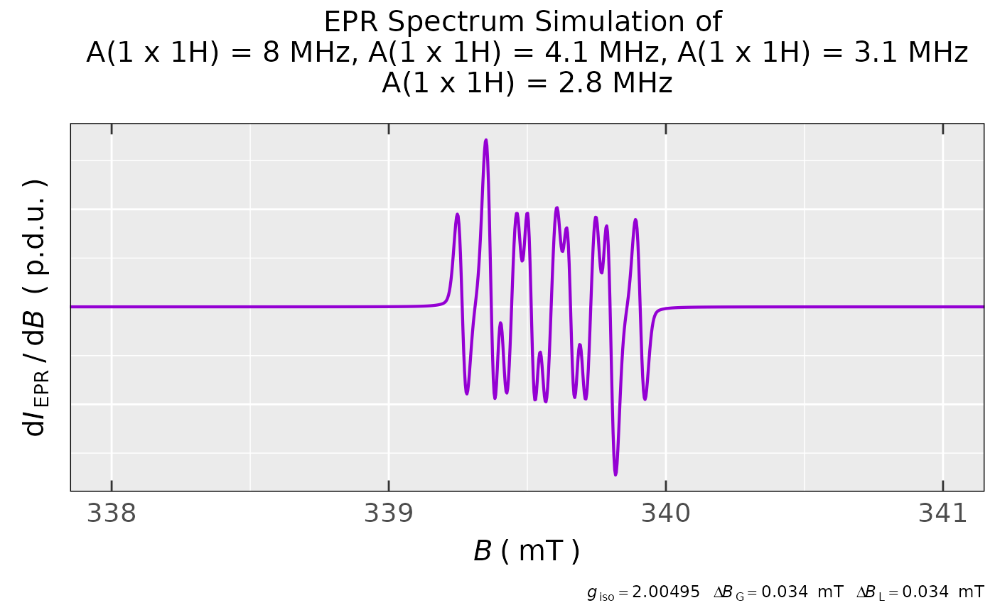
## simulation of luteolin radical anion with
## the following four hyperfine coupling constants
## A(1 x 1H) = 3.1 MHz, A(1 x 1H) = 2.8 MHz,
## A(1 x 1H) = 8.0 MHz and A(1 x 1H) = 4.1 MHz,
## one may check out the simulation
## at https://doi.org/10.1016/j.electacta.2013.06.136
## (see Fig. 6 in that article):
sim.luteol <-
eval_sim_EPR_iso(g.iso = 2.00495,
instrum.params = c(Bcf = 339.367,
Bsw = 5.9,
Npoints = 2048,
mwGHz = 9.5294),
nuclear.system = list(list("1H",1,3.1),
list("1H",1,2.8),
list("1H",1,8.0),
list("1H",1,4.1)),
lineGL.DeltaB = list(0.034,0.034),
lineG.content = 0.6,
B.unit = "mT"
)
#
## simulated spectrum preview within
## the B = (338-341) mT region:
sim.luteol$plot +
ggplot2::coord_cartesian(xlim = c(338,341))
#
## check the g_{iso}-value
## of the previous spectrum
eval_gFactor_Spec(
sim.simple.a$df,
nu.GHz = 9.8943,
Intensity = "dIeprSim_over_dB",
B = "Bsim_G"
)
#> [1] 1.9804
#
## simulation of luteolin radical anion with
## the following four hyperfine coupling constants
## A(1 x 1H) = 3.1 MHz, A(1 x 1H) = 2.8 MHz,
## A(1 x 1H) = 8.0 MHz and A(1 x 1H) = 4.1 MHz,
## one may check out the simulation
## at https://doi.org/10.1016/j.electacta.2013.06.136
## (see Fig. 6 in that article):
sim.luteol <-
eval_sim_EPR_iso(g.iso = 2.00495,
instrum.params = c(Bcf = 339.367,
Bsw = 5.9,
Npoints = 2048,
mwGHz = 9.5294),
nuclear.system = list(list("1H",1,3.1),
list("1H",1,2.8),
list("1H",1,8.0),
list("1H",1,4.1)),
lineGL.DeltaB = list(0.034,0.034),
lineG.content = 0.6,
B.unit = "mT"
)
#
## simulated spectrum preview within
## the B = (338-341) mT region:
sim.luteol$plot +
ggplot2::coord_cartesian(xlim = c(338,341))
 #
## ...and the corresponding data frame:
head(sim.luteol$df)
#> Bsim_G Bsim_mT Bsim_T dIeprSim_over_dB
#> 1 3364.170 336.4170 0.3364170 2.40049906e-06
#> 2 3364.199 336.4199 0.3364199 2.40718536e-06
#> 3 3364.228 336.4228 0.3364228 2.41389660e-06
#> 4 3364.256 336.4256 0.3364256 2.42040018e-06
#> 5 3364.285 336.4285 0.3364285 2.42716076e-06
#> 6 3364.314 336.4314 0.3364314 2.43394663e-06
#
## simulation of phenalenyl/perinaphthenyl
## (PNT) radical in the integrated form:
eval_sim_EPR_iso(g = 2.0027,
instrum.params = c(Bcf = 3500, # central field
Bsw = 100, # sweep width
Npoints = 4096,
mwGHz = 9.8), # MW Freq. in GHz
B.unit = "G",
nuclear.system = list(
list("1H",3,5.09), # 3 x A(1H) = 5.09 MHz
list("1H",6,17.67) # 6 x A(1H) = 17.67 MHz
),
lineSpecs.form = "integrated",
lineGL.DeltaB = list(0.54,NULL), # Gauss. FWHM in G
Intensity.sim = "single_Integ",
plot.sim.interact = TRUE
)
#
## simulation of methyl-viologen radical cation (MV*+)
## as reported in following papers:
## https://doi.org/10.1039/C5CP04259C (PCCP 2015)
## https://doi.org/10.1021/ja00297a006 (JACS 1985)
## https://doi.org/10.1021/j150668a021 (JPC 1984)
## https://doi.org/10.1016/0022-2364(80)90258-9
## (J MAGN RESON 1969)
## additionally, showing time (in seconds) spent
## for the computation/simulation (by the `system.time()`)
system.time(
methylViol.rad.cat.sim <-
eval_sim_EPR_iso(
g.iso = 2.0023,
instrum.params = c(
Bcf = 3400,
Bsw = 60,
Npoints = 2048,
mwGHz = 9.53
),
nuclear.system = list(
list("14N",2,11.85), # 4.23 G
list("1H",6,11.18), # 3.99 G
list("1H",4,4.46), # 1.59 G
list("1H",4,3.78) # 1.35 G
),
lineG.content = 0.5,
lineGL.DeltaB = list(0.2,0.2)
)
)
#> user system elapsed
#> 0.17 0.00 0.17
#
## simulated spectrum of MV*+
methylViol.rad.cat.sim$plot +
ggplot2::coord_cartesian(
xlim = c(3373,3427)
)
#
## ...and the corresponding data frame:
head(sim.luteol$df)
#> Bsim_G Bsim_mT Bsim_T dIeprSim_over_dB
#> 1 3364.170 336.4170 0.3364170 2.40049906e-06
#> 2 3364.199 336.4199 0.3364199 2.40718536e-06
#> 3 3364.228 336.4228 0.3364228 2.41389660e-06
#> 4 3364.256 336.4256 0.3364256 2.42040018e-06
#> 5 3364.285 336.4285 0.3364285 2.42716076e-06
#> 6 3364.314 336.4314 0.3364314 2.43394663e-06
#
## simulation of phenalenyl/perinaphthenyl
## (PNT) radical in the integrated form:
eval_sim_EPR_iso(g = 2.0027,
instrum.params = c(Bcf = 3500, # central field
Bsw = 100, # sweep width
Npoints = 4096,
mwGHz = 9.8), # MW Freq. in GHz
B.unit = "G",
nuclear.system = list(
list("1H",3,5.09), # 3 x A(1H) = 5.09 MHz
list("1H",6,17.67) # 6 x A(1H) = 17.67 MHz
),
lineSpecs.form = "integrated",
lineGL.DeltaB = list(0.54,NULL), # Gauss. FWHM in G
Intensity.sim = "single_Integ",
plot.sim.interact = TRUE
)
#
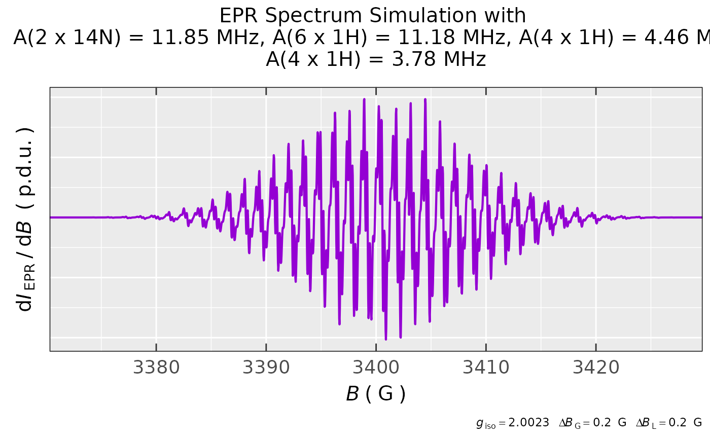
## simulation of methyl-viologen radical cation (MV*+)
## as reported in following papers:
## https://doi.org/10.1039/C5CP04259C (PCCP 2015)
## https://doi.org/10.1021/ja00297a006 (JACS 1985)
## https://doi.org/10.1021/j150668a021 (JPC 1984)
## https://doi.org/10.1016/0022-2364(80)90258-9
## (J MAGN RESON 1969)
## additionally, showing time (in seconds) spent
## for the computation/simulation (by the `system.time()`)
system.time(
methylViol.rad.cat.sim <-
eval_sim_EPR_iso(
g.iso = 2.0023,
instrum.params = c(
Bcf = 3400,
Bsw = 60,
Npoints = 2048,
mwGHz = 9.53
),
nuclear.system = list(
list("14N",2,11.85), # 4.23 G
list("1H",6,11.18), # 3.99 G
list("1H",4,4.46), # 1.59 G
list("1H",4,3.78) # 1.35 G
),
lineG.content = 0.5,
lineGL.DeltaB = list(0.2,0.2)
)
)
#> user system elapsed
#> 0.17 0.00 0.17
#
## simulated spectrum of MV*+
methylViol.rad.cat.sim$plot +
ggplot2::coord_cartesian(
xlim = c(3373,3427)
)