Least-Squares Fitting of Isotropic EPR Spectra by Simulations
Source:R/eval_sim_EPR_isoFit.R
eval_sim_EPR_isoFit.RdFitting of the simulated spectrum onto the experimental one represents an important step in the analysis
of EPR spectra. Parameters of the simulated spectrum like \(g_{\text{iso}}\); coupling constants
(in MHz) \(A_{\text{iso}}\) for each group of equivalent nuclei; linewidth
(either \(\Delta B_{\text{pp}}\) or \(FWHM\) depending on the lineSpecs.form argument);
spectral baseline (see the baseline.correct argument) and finally the intensity (multiplication coefficient)
are optimized by the methods listed in optim_for_EPR_fitness.
The lineG.content corresponding parameter is the only one,
which needs to be varied "manually". For an extended version of this function
(including automatic lineG.content variations), please refer to the eval_sim_EPR_isoFit_space.
Usage
eval_sim_EPR_isoFit(
  data.spectr.expr,
  Intensity.expr = "dIepr_over_dB",
  Intensity.sim = "dIeprSim_over_dB",
  nu.GHz,
  B.unit = "G",
  Blim = NULL,
  nuclear.system.noA = NULL,
  baseline.correct = "constant",
  lineG.content = 0.5,
  lineSpecs.form = "derivative",
  optim.method = "neldermead",
  optim.params.init,
  optim.params.fix.id = NULL,
  optim.params.lower = NULL,
  optim.params.upper = NULL,
  Nmax.evals = 512,
  check.fit.plot = TRUE,
  msg.optim.progress = TRUE,
  output.list.forFitSp = FALSE,
  ...
)
Arguments
- data.spectr.expr
Data frame object/table, containing the experimental spectral data with the magnetic flux density (
"B_mT"or"B_G") and the intensity (see theIntensity.exprargument) columns.- Intensity.expr
Character string, pointing to column name of the experimental EPR intensity within the original
data.spectr.expr. Default:dIepr_over_dB.- Intensity.sim
Character string, pointing to column name of the simulated EPR intensity within the related output data frame. Default:
Intensity.sim = "dIeprSim_over_dB".- nu.GHz
Numeric value, microwave frequency in
GHz.- B.unit
Character string, denoting the magnetic flux density unit e.g.
B.unit = "G"(gauss, default) orB.unit = "mT"/"T"(millitesla/tesla).- Blim
Numeric vector, magnetic flux density in
mT/Gcorresponding to lower and upper visual limit of the selected \(B\)-region, such asBlim = c(3495.4,3595.4). Default:Blim = NULL(corresponding to the entire \(B\)-range of EPR spectrum). This does not correspond to simulation fit data region !. If narrower \(B\)-region (in comparison to the original one) is required to fit the EPR spectrum, the filtering has to be done prior to own fitting procedure. For example, if the original data frame (df.spectr.orginwithin 200 G), of the experimental EPR spectrum, should be fitted within the region ofB = c(3450,3550)(100 G), following operation must be performed:df.spectr.actuall <- df.spectr.origin |> dplyr::filter(dplyr::between(B_G,3450,3550)), where thedf.spectr.actuallserves as an input (represented by thedata.spectr.exprargument) for the function.- nuclear.system.noA
List or nested list without estimated hyperfine coupling constant values, such as
list("14N",1)orlist(list("14N", 2),list("1H", 4),list("1H", 12)). The \(A\)-values are already defined as elements of theoptim.params.initargument/vector. If the EPR spectrum does not display any hyperfine splitting, the argument definition readsnuclear.system.noA = NULL(default).- baseline.correct
Character string, referring to baseline correction of the simulated/fitted spectrum. Corrections like
"constant"(default),"linear"or"quadratic"can be applied.- lineG.content
Numeric value between
0and1, referring to content of the Gaussian line form. IflineG.content = 1(default) it corresponds to "pure" Gaussian line form and iflineG.content = 0it corresponds to Lorentzian one. The value from (0,1) (e.g.lineG.content = 0.5) represents the linear combination (for the example above, with the coefficients 0.5 and 0.5) of both line forms => so called pseudo-Voigt.- lineSpecs.form
Character string, describing either
"derivative"(default) or"integrated"(i.e."absorption"which can be used as well) line form of the analyzed EPR spectrum/data.- optim.method
Character string (vector), setting the optimization method(s) gathered within the
optim_for_EPR_fitness. Default:optim.method = "neldermead". Additionally, several consecutive methods can be defined likeoptim.method = c("levenmarq","neldermead"), where the best fit parameters from the previous method are used as input for the next one. In such case, the output islistwith the elements/vectors from each method, in order to see the progress of the optimization.- optim.params.init
Numeric vector with the initial parameter guess (elements) where the first five elements are immutable
g-value (g-factor)
Gaussian linewidth
Lorentzian linewidth
baseline constant (intercept or offset)
intensity multiplication constant
baseline slope (only if
baseline.correct = "linear"orbaseline.correct = "quadratic"), ifbaseline.correct = "constant"it corresponds to the first HFCC (\(A_1\))baseline quadratic coefficient (only if
baseline.correct = "quadratic"), ifbaseline.correct = "constant"it corresponds to the second HFCC (\(A_2\)), ifbaseline.correct = "linear"it corresponds to the first HFCC (\(A_1\))additional HFCC (\(A_3\)) if
baseline.correct = "constant"or ifbaseline.correct = "linear"(\(A_2\)), ifbaseline.correct = "quadratic"it corresponds to the first HFCC (\(A_1\))...additional HFCCs (\(A_k...\), each vector element is reserved only for one \(A\))
DO NOT PUT ANY OF THESE PARAMETERS to
NULL. If the lineshape is expected to be pure Lorentzian or pure Gaussian then put the corresponding vector element to0.- optim.params.fix.id
Numeric value/vector of index/indices of the
optim.params.init, corresponding to optimization/simulation parameter(s) to be fixed. For example, if the g-Value and the (intensity) multiplication constant should not be optimized (their values should be fixed during the procedure), the argument must be defined as follows:optim.params.fix.id = c(1,5)(see also theoptim.params.initdescription for the simulation/optimized parameters order). Default:optim.params.fix.id = NULL, indicating that none of theoptim.params.initis fixed, i.e. all parameters are optimized within their default/defined boundaries (see theoptim.params.lowerand theoptim.params.upper). Alternatively, the parameter value(s) can be also adjusted by assigning theoptim.params.init+optim.params.lower+optim.params.upperelements to the same value, as already demonstrated in theExamples.- optim.params.lower
Numeric vector (with the same element order like
optim.params.init) with the lower bound constraints. Default:optim.params.lower = NULLwhich actually equals to \(g_{\text{init}} - 0.001\), \(0.8\,\Delta B_{\text{G,init}}\), \(0.8\,\Delta B_{\text{L,init}}\), baseline intercept initial constant \(- 0.001\), intensity multiplication initial constant \(= 0.75\,\text{init}\), baseline initial slope \(- 5\) (in case thebaseline.correctis set either to"linear"or"quadratic") and finally, the baseline initial quadratic coefficient \(- 5\) (in case thebaseline.correctis set to"quadratic"). Default lower limits of all hyperfine coupling constant (HFCCs) are set to \(0.875\,A_{\text{init}}\).- optim.params.upper
Numeric vector (with the same element order like
optim.params.init) with the upper bound constraints. Default:optim.params.upper = NULLwhich actually equals to \(g_{\text{init}} + 0.001\), \(1.2\,\Delta B_{\text{G,init}}\), \(1.2\,\Delta B_{\text{L,init}}\), baseline intercept initial constant \(+ 0.001\), intensity multiplication initial constant \(= 1.25\,\text{init}\), baseline initial slope \(+ 5\) (in case thebaseline.correctis set either to"linear"or"quadratic") and finally, the baseline initial quadratic coefficient \(+ 5\) (in case thebaseline.correctis set to"quadratic"). Default upper limits of all HFCCs are set to \(1.125\,A_{\text{init}}\).- Nmax.evals
Numeric value, maximum number of function evaluations and/or iterations. The only one method, limited by this argument, is
nls.lm, whereNmax.evals = 1024. HigherNmax.evalsmay extremely extend the optimization time, therefore the default value readsNmax.evals = 512. However, the"pswarm"method requires at least the default or even higher values.- check.fit.plot
Logical, whether to return overlay plot with the initial simulation + the best simulation fit + experimental spectrum (including residuals in the lower part of the plot,
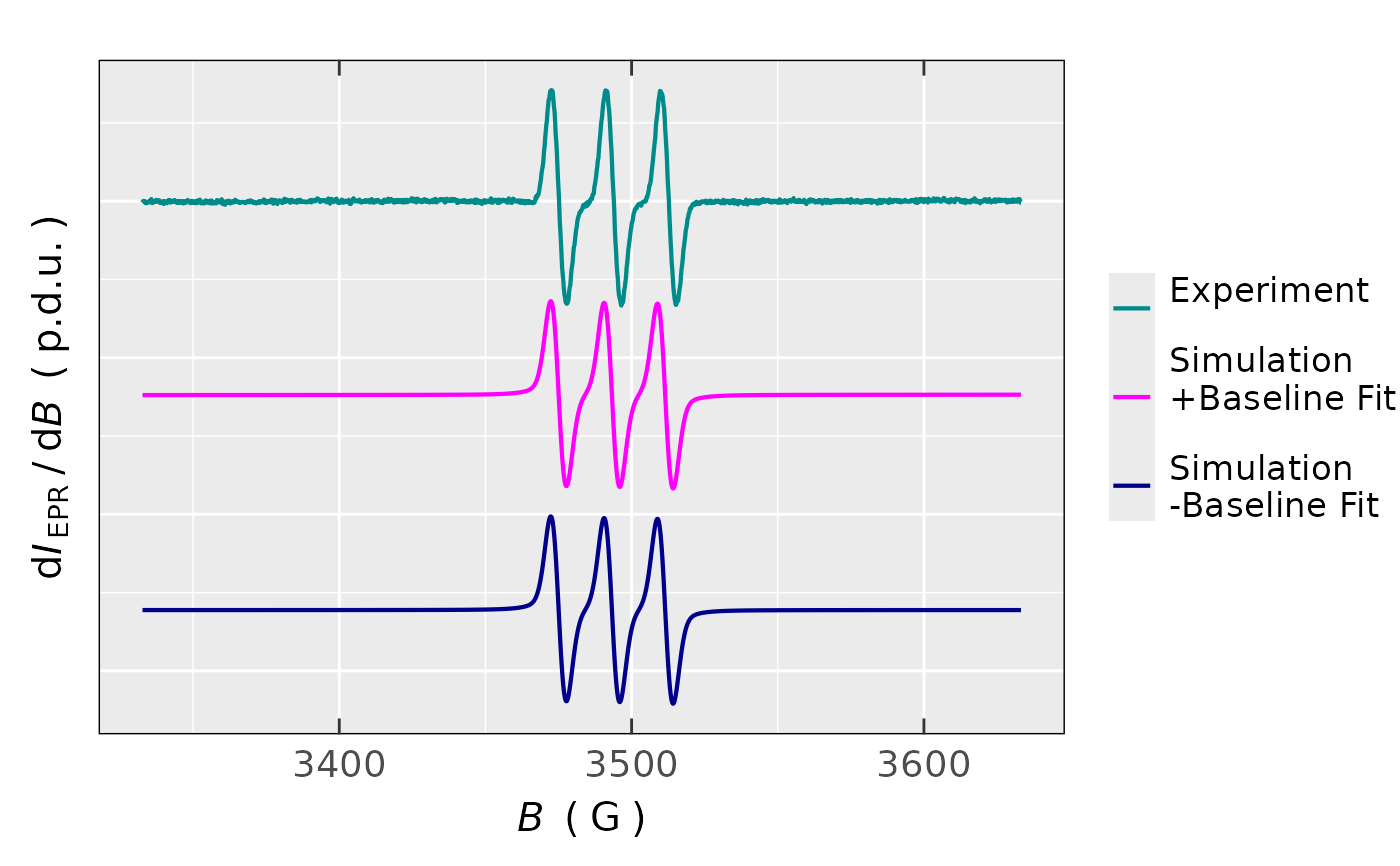
check.fit.plot = TRUE, default) or with the following three spectra (check.fit.plot = FALSE): 1. experimental, 2. the best simulated one with the baseline fit and 3. the best simulated spectrum with the baseline fit subtracted. The latter two are offset for clarity, within the plot.- msg.optim.progress
Logical, whether to display message (in the R console) about progress of the
optim.methodduring the optimization/fitting procedure, e.g."EPR simulation parameters are currently being optimized by NELDERMEAD, method 1 of 2..."and at the end it shows the elapsed time. Default:msg.optim.progress = TRUE. IfFALSE, no message is displayed. Latter option is especially suitable for the case whenoutput.list.forFitSp = TRUE(see below). This argument can be combined with the optionaleval.optim.progress(see below or described in theoptim_for_EPR_fitness).- output.list.forFitSp
Logical. If
TRUE,listwith the following components will be exclusively returned: 1. optimized parameters from the best fit (together with the minimum sum of residual squares) and 2. Plot of the experimental as well as simulated EPR spectrum depending oncheck.fit.plot(seeValue). Such output is applied for theeval_sim_EPR_isoFit_space, therefore, the default value readsoutput.list.final = FALSE.- ...
additional arguments specified, see also
optim_for_EPR_fitness, likeeval.optim.progress = TRUE(which isFALSEby default),pswarm.size,pswarm.diameter,pswarm.type,tol.step+optim.methoddepended additional arguments.
Value
Optimization/Fitting procedure results in vector or data frame or list depending on the check.fit.plot
and output... arguments.
If
check.fit.plot = TRUEorcheck.fit.plot = FALSE, the result corresponds to list with the following components:- plot
Visualization of the experimental as well as the best fitted EPR simulated spectra. If
check.fit.plot = TRUE, the overlay plot consists of the initial simulation + the best simulation fit + experimental spectrum, including residuals in the plot lower part. Whereas, ifcheck.fit.plot = FALSE, following three spectra are available: 1. experimental, 2. the best simulated one with the baseline fit and 3. the best simulated spectrum with the baseline fit subtracted. The latter two are offset for clarity.- ra
Simple residual analysis - a list consisting of 4 elements: diagnostic plots
plot.rqq()function,plot.histDens; original data frame (df) with residuals and their corresponding standard deviation (sd). For details, please refer to theplot_eval_RA_forFit.- best.fit.params
Vector of the best (final) fitting (optimized) parameters, for each corresponding
optim.method, to simulate the experimental EPR spectrum, see also description of theoptim.params.init.- df
Tidy data frame (table) with the magnetic flux density and intensities of the experimental, the best simulated/fitted, as well as the initially simulated EPR spectrum and residuals (if
check.fit.plot = TRUE), or wide data frame with the following variables / columns (forcheck.fit.plot = FALSE): magnetic flux density, intensity of the experimental spectrum, intensity of the best simulated one (including the baseline fit), residual intensity and finally, the best simulated spectrum intensity without the baseline fit.- min.rss
Minimum sum of residual squares (vector) after the least-square procedure.
- cov.df
Covariance
matrixof a data frame, consisting of EPR experimental, simulated (best fit) and the residual intensities as columns/variables. Covariance between the experiment and simulation should be positive and strong for a decent fit. Contrary, thecovbetween the simulation and residuals should be ideally close to0, indicating no systematic relationship. However, the covariance is scale-depended and must be "normalized". Therefore, for such a purpose, the correlation is defined as shown below.- cor.df
Correlation
matrixof a data frame, consisting of EPR experimental, simulated (best fit) and residual intensities as columns/variables. Such matrix can be additionally nicely visualized by a correlationplotcreated by thecorrplotfunction. A higher positive correlation (between the experiment and the best fit), with the value close to1, indicates that simulation best fit nicely follows the experimental spectrum. Contrary, no clear correlation between the residuals and the experimental/fitted EPR intensities must be visible. Therefore, such correlation should be ideally close to0.- abic
A list consisting of Akaike and Bayesian information criteria (AIC & BIC) vector (
abic.vec) andmessage, denoting the residuals/errors distribution, applied to evaluate those criteria. To be used when comparing different simulation fits. The lower the (negative) values, the better the fit. Please, refer to theeval_ABIC_forFit.- N.evals
Number of iterations/function evaluations completed before termination. If the
pswarmoptimization algorithm is included inoptim.method, theN.evalsequals to vector with the following elements: number of function evaluations, number of iterations (per one particle) and the number of restarts.- N.converg
Vector or simple integer code indicating the successful completion of the optimization/fit. In the case of
"levenmarq"method, the vector elements coincide with the sum of residual squares at each iteration. If theoptim.method = "pswarm"is applied, one of the following codes can be returned:0: algorithm terminated by reaching the absolute tolerance,1: maximum number of function evaluations reached,2: maximum number of iterations reached,3: maximum number of restarts reached,4: maximum number of iterations without improvement reached. For all the other remaining methods (coming from{nloptr}package), the integers have to be positive to indicate successful convergence.
If
output.list.forFitSp = TRUE, the function exclusively returns list with the two components, which is to be applied for theeval_sim_EPR_isoFit_space.- params
A vector, containing the following elements:
The best fitting (optimized) parameters (related to the
optim.params.initargument).Minimum sum of residual squares (corresponding to previous item).
Standard deviation of residuals, after the (final)
optim.methodprocedure.Akaike Information Criterion/AIC metric (refer to
eval_ABIC_forFit), after the (final)optim.method.Bayesian Information Criterion/BIC metric (refer to
eval_ABIC_forFit), after the (final)optim.method.
- plot
Visualization of the experimental as well as the best fitted EPR simulated spectra depending on the
check.fit.plot. It corresponds either to EPR spectra with residuals or to those with baseline correction, (please, refer to thecheck.fit.plotargument description).
Note
In order to guess the intensity multiplication constant (please, refer to the optim.params.init
argument), one might compare the intensities of the experimental (expr) and simulated (sim)
EPR spectrum by one of the interactive or static plot functions (e.g. plot_EPR_Specs
or plot_EPR_Specs2D_interact) as well as by the eval_sim_EPR_iso. Accordingly,
the initial intensity multiplication constant can be estimated as the ratio
max(expr intensity)/max(sim intensity) * 0.25. The coefficient 0.25(1/4) is
introduced in order to be sure that both of the experimental and initially simulated EPR spectra,
in the graphical output (see the Value), are clearly visible if check.fit.plot = TRUE.
Otherwise, the spectra may overlay and it will be difficult to differentiate between them. Of course,
any intensity multiplication coefficient, close to the experimental EPR intensity, can be applied as a starting
point to evaluate the fit.
To fix one or more simulation parameter(s) (i.e. parameter(s) which is/are not optimized) during
the fitting procedure, the corresponding optim.parms.lower as well as the optim.params.upper vector
element(s) must equal to that of the optim.params.init. Please, refer to the Examples below
for the simulation fit of aminoxyl radical EPR spectrum with bound constraints and fixed A(1 x 14N).
An alternative selection of a non-optimized/fixed simulation parameter can be also done by using
the optim.params.fix.id argument, which can be also applied to fix the simulation parameters when searching
for the best fit by the eval_sim_EPR_isoFit_space. Therefore, the latter function argument just selects
an element of the optim.params.init (by its corresponding index) and accordingly, the selected simulation
parameter value won't be optimized.
A simple EPR spectrum analysis by interactive simulation using the plot_eval_ExpSim_app
may return an .R script/code snippet for the initial simulation fit and therefore
the user does not have to write (or remember) the code required to run the eval_sim_EPR_isoFit.
Rather, she/he can instantly and seamlessly analyze an isotropic EPR spectrum by optimizing the simulation parameters.
Examples
## loading built-in example dataset which is simple
## EPR spectrum of the aminoxyl radical:
aminoxyl.data.path <-
load_data_example(file = "Aminoxyl_radical_a.DTA")
aminoxyl.data <-
readEPR_Exp_Specs(
path_to_file = aminoxyl.data.path,
qValue = 2100
)
#
## EPR spectrum simulation fit with "Nelder-Mead"
## optimization method with `check.fit.plot = FALSE`:
tempo.test.sim.fit.a <-
eval_sim_EPR_isoFit(data.spectr.expr = aminoxyl.data,
nu.GHz = 9.806769,
lineG.content = 0.5,
optim.method = "neldermead",
nuclear.system.noA = list("14N",1),
baseline.correct = "linear",
optim.params.init =
c(2.006, # g-value
4.8, # G Delta Bpp
4.8, # L Delta Bpp
0, # intercept (constant) lin. baseline
0.018, # Sim. intensity multiply
1e-6, # slope lin. baseline
49), # A in MHz
check.fit.plot = FALSE,
msg.optim.progress = FALSE
)
## OUTPUTS:
## best fit parameters:
tempo.test.sim.fit.a$best.fit.params
#> [[1]]
#> [1] 2.0059448e+00 5.4974114e+00 5.1862704e+00 -9.4929049e-05 1.8070618e-02
#> [6] 2.7243216e-08 5.1351972e+01
#>
#
## spectrum plot with experimental spectrum,
## simulated one with the linear baseline fit
## and simulated one with the linear baseline
## fit subtracted:
tempo.test.sim.fit.a$plot
 #
## minimum sum of residual squares:
tempo.test.sim.fit.a$min.rss
#> [[1]]
#> [1] 3.3805427e-07
#>
#
## number of evaluations / iterations:
tempo.test.sim.fit.a$N.evals
#> [[1]]
#> [1] 512
#>
#
## convergence, in this case it is represented
## by the integer code indicating the successful
## completion (it must be > 0):
tempo.test.sim.fit.a$N.converg
#> [[1]]
#> [1] 5
#>
#
## preview of data frame including all EPR spectra:
head(tempo.test.sim.fit.a$df)
#> B_G Experiment Simulation Residuals Simulation_NoBasLin
#> 1 3332.7000 -1.7738564e-06 -4.1290221e-06 2.3551657e-06 6.5629077e-09
#> 2 3332.9005 1.2209461e-07 -4.1235480e-06 4.2456426e-06 6.5756338e-09
#> 3 3333.1009 -1.8403788e-07 -4.1180464e-06 3.9340085e-06 6.6158641e-09
#> 4 3333.3014 -7.1641412e-08 -4.1125720e-06 4.0409306e-06 6.6288572e-09
#> 5 3333.5019 -1.7361444e-06 -4.1070702e-06 2.3709258e-06 6.6693576e-09
#> 6 3333.7023 -5.1531169e-07 -4.1015956e-06 3.5862839e-06 6.6826214e-09
#
## similar EPR spectrum simulation fit with "particle swarm"
## optimization algorithm and `check.fit.plot = TRUE` option
## as well as user defined bound constraints, including
## fixed A(1 x 14N) = 52.6 MHz:
tempo.test.sim.fit.b <-
eval_sim_EPR_isoFit(data.spectr.expr = aminoxyl.data,
nu.GHz = 9.806769,
lineG.content = 0.75,
optim.method = "pswarm",
nuclear.system.noA = list("14N",1),
baseline.correct = "constant",
optim.params.init = c(2.0062,4.8,4.8,0,8e-3,52.68),
optim.params.lower = c(2.0048,4.6,4.6,-1e-4,5e-3,52.68),
optim.params.upper = c(2.0068,5.0,5.0,1e-4,1.5e-2,52.68),
check.fit.plot = TRUE,
eval.optim.progress = TRUE ## iterations, progress
)
#>
#>
EPR simulation parameters are currently being optimized by PSWARM ; method 1 of 1 ...
#> S=14, K=6, p=0.359, w0=0.7213, w1=0.7213, c.p=1.193, c.g=1.193
#> v.max=NA, d=0.5658, vectorize=FALSE, hybrid=off
#> It 10: fitness=3.395e-08, swarm diam.=0.2458
#> It 20: fitness=1.88e-08, swarm diam.=0.1672
#> It 30: fitness=1.507e-08, swarm diam.=0.05766
#> Maximal number of function evaluations reached
#>
#>
Done! ( 100 %) elapsed time 12.273 s
## OUTPUTS:
## minimum sum of residual squares:
tempo.test.sim.fit.b$min.rss
#> [[1]]
#> [1] 1.4847253e-08
#>
#
## check and compare the previous value
## by residual analysis (`ra`)
sum((tempo.test.sim.fit.b$ra$df$Residuals)^2)
#> [1] 1.4847253e-08
#
## number of evaluations / iterations:
tempo.test.sim.fit.b$N.evals
#> [[1]]
#> function iteration restarts
#> 512 37 0
#>
#
## best fit parameters:
tempo.test.sim.fit.b$best.fit.params
#> [[1]]
#> [1] 2.0053059e+00 4.9990459e+00 4.8001383e+00 1.2503903e-07 1.2912288e-02
#> [6] 5.2680000e+01
#>
#
## correlation matrix of the EPR simulation fit:
tempo.test.sim.fit.b$cor.df
#> Experiment Simulation Residuals
#> Experiment 1.000000000 0.995689842 0.048364255
#> Simulation 0.995689842 1.000000000 -0.044481227
#> Residuals 0.048364255 -0.044481227 1.000000000
#
## visualization of the previous matrix:
tempo.test.sim.fit.b$cor.df %>%
corrplot::corrplot(addCoef.col = "#c2c2c2")
#
## minimum sum of residual squares:
tempo.test.sim.fit.a$min.rss
#> [[1]]
#> [1] 3.3805427e-07
#>
#
## number of evaluations / iterations:
tempo.test.sim.fit.a$N.evals
#> [[1]]
#> [1] 512
#>
#
## convergence, in this case it is represented
## by the integer code indicating the successful
## completion (it must be > 0):
tempo.test.sim.fit.a$N.converg
#> [[1]]
#> [1] 5
#>
#
## preview of data frame including all EPR spectra:
head(tempo.test.sim.fit.a$df)
#> B_G Experiment Simulation Residuals Simulation_NoBasLin
#> 1 3332.7000 -1.7738564e-06 -4.1290221e-06 2.3551657e-06 6.5629077e-09
#> 2 3332.9005 1.2209461e-07 -4.1235480e-06 4.2456426e-06 6.5756338e-09
#> 3 3333.1009 -1.8403788e-07 -4.1180464e-06 3.9340085e-06 6.6158641e-09
#> 4 3333.3014 -7.1641412e-08 -4.1125720e-06 4.0409306e-06 6.6288572e-09
#> 5 3333.5019 -1.7361444e-06 -4.1070702e-06 2.3709258e-06 6.6693576e-09
#> 6 3333.7023 -5.1531169e-07 -4.1015956e-06 3.5862839e-06 6.6826214e-09
#
## similar EPR spectrum simulation fit with "particle swarm"
## optimization algorithm and `check.fit.plot = TRUE` option
## as well as user defined bound constraints, including
## fixed A(1 x 14N) = 52.6 MHz:
tempo.test.sim.fit.b <-
eval_sim_EPR_isoFit(data.spectr.expr = aminoxyl.data,
nu.GHz = 9.806769,
lineG.content = 0.75,
optim.method = "pswarm",
nuclear.system.noA = list("14N",1),
baseline.correct = "constant",
optim.params.init = c(2.0062,4.8,4.8,0,8e-3,52.68),
optim.params.lower = c(2.0048,4.6,4.6,-1e-4,5e-3,52.68),
optim.params.upper = c(2.0068,5.0,5.0,1e-4,1.5e-2,52.68),
check.fit.plot = TRUE,
eval.optim.progress = TRUE ## iterations, progress
)
#>
#>
EPR simulation parameters are currently being optimized by PSWARM ; method 1 of 1 ...
#> S=14, K=6, p=0.359, w0=0.7213, w1=0.7213, c.p=1.193, c.g=1.193
#> v.max=NA, d=0.5658, vectorize=FALSE, hybrid=off
#> It 10: fitness=3.395e-08, swarm diam.=0.2458
#> It 20: fitness=1.88e-08, swarm diam.=0.1672
#> It 30: fitness=1.507e-08, swarm diam.=0.05766
#> Maximal number of function evaluations reached
#>
#>
Done! ( 100 %) elapsed time 12.273 s
## OUTPUTS:
## minimum sum of residual squares:
tempo.test.sim.fit.b$min.rss
#> [[1]]
#> [1] 1.4847253e-08
#>
#
## check and compare the previous value
## by residual analysis (`ra`)
sum((tempo.test.sim.fit.b$ra$df$Residuals)^2)
#> [1] 1.4847253e-08
#
## number of evaluations / iterations:
tempo.test.sim.fit.b$N.evals
#> [[1]]
#> function iteration restarts
#> 512 37 0
#>
#
## best fit parameters:
tempo.test.sim.fit.b$best.fit.params
#> [[1]]
#> [1] 2.0053059e+00 4.9990459e+00 4.8001383e+00 1.2503903e-07 1.2912288e-02
#> [6] 5.2680000e+01
#>
#
## correlation matrix of the EPR simulation fit:
tempo.test.sim.fit.b$cor.df
#> Experiment Simulation Residuals
#> Experiment 1.000000000 0.995689842 0.048364255
#> Simulation 0.995689842 1.000000000 -0.044481227
#> Residuals 0.048364255 -0.044481227 1.000000000
#
## visualization of the previous matrix:
tempo.test.sim.fit.b$cor.df %>%
corrplot::corrplot(addCoef.col = "#c2c2c2")
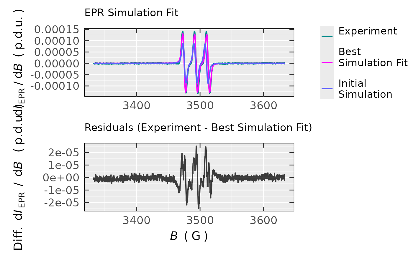 #
## quick simulation check by plotting the both
## simulated and the experimental EPR spectra
## together with the initial simulation
## and the residuals (differences between the
## experiment and the best fit)
tempo.test.sim.fit.b$plot
#
## quick simulation check by plotting the both
## simulated and the experimental EPR spectra
## together with the initial simulation
## and the residuals (differences between the
## experiment and the best fit)
tempo.test.sim.fit.b$plot
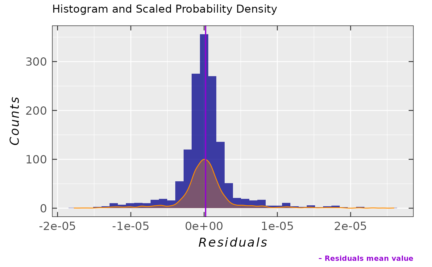 #
## simple residual density plot
## together with standard deviation
tempo.test.sim.fit.b$ra$plot.histDens
#
## simple residual density plot
## together with standard deviation
tempo.test.sim.fit.b$ra$plot.histDens
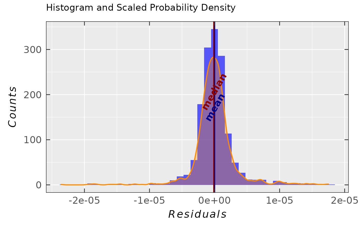 tempo.test.sim.fit.b$ra$sd
#> [1] 3.1524467e-06
#
## Akaike and Bayesian Criteria (AIC & BIC)
## + information about the residuals distribution
tempo.test.sim.fit.b$abic
#> $abic.vec
#> [1] -34005.133 -33978.607
#>
#> $message
#> [1] "Information criteria evaluated using the"
#> [2] "Student's t-distribution of residuals with 6"
#> [3] "degrees of freedom. Additionally supported"
#> [4] "by the Shapiro-Wilk as well as by the"
#> [5] "Kolmogorov-Smirnov tests."
#>
#
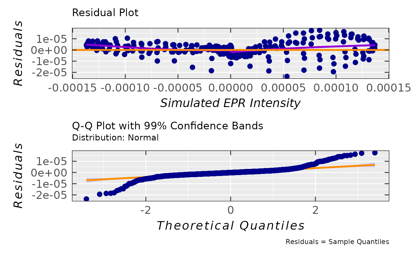
## residual & Q-Q plots for the proposed normal
## distribution of residuals and confidence level 99%
## (default: 95%/0.95)
tempo.test.sim.fit.b$ra$plot.rqq(confidence = 0.99)
#> `geom_smooth()` using method = 'gam' and formula = 'y ~ s(x, bs = "cs")'
tempo.test.sim.fit.b$ra$sd
#> [1] 3.1524467e-06
#
## Akaike and Bayesian Criteria (AIC & BIC)
## + information about the residuals distribution
tempo.test.sim.fit.b$abic
#> $abic.vec
#> [1] -34005.133 -33978.607
#>
#> $message
#> [1] "Information criteria evaluated using the"
#> [2] "Student's t-distribution of residuals with 6"
#> [3] "degrees of freedom. Additionally supported"
#> [4] "by the Shapiro-Wilk as well as by the"
#> [5] "Kolmogorov-Smirnov tests."
#>
#
## residual & Q-Q plots for the proposed normal
## distribution of residuals and confidence level 99%
## (default: 95%/0.95)
tempo.test.sim.fit.b$ra$plot.rqq(confidence = 0.99)
#> `geom_smooth()` using method = 'gam' and formula = 'y ~ s(x, bs = "cs")'
 #
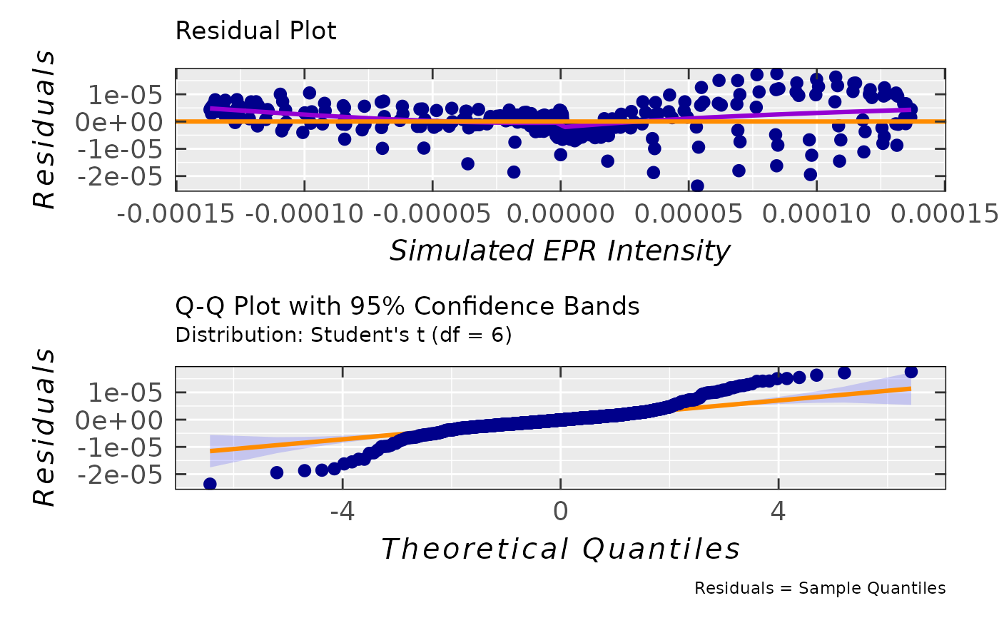
## residual & Q-Q plots for the proposed Student's
## distribution of residuals with degrees of freedom
## df = 6 (see the "$message" right above)
tempo.test.sim.fit.b$ra$plot.rqq(
residuals.distro = "t",
df = 6
)
#> `geom_smooth()` using method = 'gam' and formula = 'y ~ s(x, bs = "cs")'
#
## residual & Q-Q plots for the proposed Student's
## distribution of residuals with degrees of freedom
## df = 6 (see the "$message" right above)
tempo.test.sim.fit.b$ra$plot.rqq(
residuals.distro = "t",
df = 6
)
#> `geom_smooth()` using method = 'gam' and formula = 'y ~ s(x, bs = "cs")'
 #
## fitting of the aminoxyl EPR spectrum
## by the combination of the 1. "Levenberg-Marquardt"
## and 2. "Nelder-Mead" algorithms
tempo.test.sim.fit.c <-
eval_sim_EPR_isoFit(aminoxyl.data,
nu.GHz = 9.86769,
lineG.content = 0.5,
optim.method = c("levenmarq",
"neldermead"),
nuclear.system.noA = list("14N",1),
baseline.correct = "constant",
optim.params.init = c(2.0060,
4.8,
4.8,
0,
7e-3,
49),
check.fit.plot = FALSE
)
#>
#>
EPR simulation parameters are currently being optimized by LEVENMARQ ; method 1 of 2 ...
#>
#>
Done! ( 50 %) elapsed time 0.793 s
#>
#>
EPR simulation parameters are currently being optimized by NELDERMEAD ; method 2 of 2 ... ...
#>
#>
Done! ( 100 %) elapsed time 12.227 s
## OUTPUTS:
## best fit parameters for both procedures within a list:
tempo.test.sim.fit.c$best.fit.params
#> [[1]]
#> [1] 2.0060000e+00 5.7600000e+00 5.7600000e+00 -4.9940834e-10 6.4310899e-03
#> [6] 4.9000000e+01
#>
#> [[2]]
#> [1] 2.0069998e+00 4.8414479e+00 3.8400101e+00 -1.7672999e-09 8.7499986e-03
#> [6] 5.3612524e+01
#>
#
## compare the results with the example in the `readMAT_params_file`,
## corresponding to the best fit from `Easyspin`
#
## `N.converg` also consists of two components
## each corresponding to result of the individual
## optimization method where the "levenmarq" returns
## the sum of squares at each iteration, therefore the 1st
## component is vector and the 2nd one is integer code
## as already stated above:
tempo.test.sim.fit.c$N.converg
#> [[1]]
#> [1] 1.6573191e-06 1.5727024e-06 1.5529725e-06 1.5518805e-06 1.5518805e-06
#>
#> [[2]]
#> [1] 5
#>
#
## Akaike and Bayesian Criteria (AIC & BIC)
## + information about the residuals distribution
tempo.test.sim.fit.c$abic
#> $abic.vec
#> [1] -27866.027 -27834.204
#>
#> $message
#> [1] "Information criteria evaluated using the"
#> [2] "Student's t-distribution of residuals with 4"
#> [3] "degrees of freedom. Additionally supported"
#> [4] "by the Shapiro-Wilk as well as by the"
#> [5] "Kolmogorov-Smirnov tests."
#>
#
## fitting of the aminoxyl EPR spectrum
## by the combination of the 1. "Levenberg-Marquardt"
## and 2. "Nelder-Mead" algorithms
tempo.test.sim.fit.c <-
eval_sim_EPR_isoFit(aminoxyl.data,
nu.GHz = 9.86769,
lineG.content = 0.5,
optim.method = c("levenmarq",
"neldermead"),
nuclear.system.noA = list("14N",1),
baseline.correct = "constant",
optim.params.init = c(2.0060,
4.8,
4.8,
0,
7e-3,
49),
check.fit.plot = FALSE
)
#>
#>
EPR simulation parameters are currently being optimized by LEVENMARQ ; method 1 of 2 ...
#>
#>
Done! ( 50 %) elapsed time 0.793 s
#>
#>
EPR simulation parameters are currently being optimized by NELDERMEAD ; method 2 of 2 ... ...
#>
#>
Done! ( 100 %) elapsed time 12.227 s
## OUTPUTS:
## best fit parameters for both procedures within a list:
tempo.test.sim.fit.c$best.fit.params
#> [[1]]
#> [1] 2.0060000e+00 5.7600000e+00 5.7600000e+00 -4.9940834e-10 6.4310899e-03
#> [6] 4.9000000e+01
#>
#> [[2]]
#> [1] 2.0069998e+00 4.8414479e+00 3.8400101e+00 -1.7672999e-09 8.7499986e-03
#> [6] 5.3612524e+01
#>
#
## compare the results with the example in the `readMAT_params_file`,
## corresponding to the best fit from `Easyspin`
#
## `N.converg` also consists of two components
## each corresponding to result of the individual
## optimization method where the "levenmarq" returns
## the sum of squares at each iteration, therefore the 1st
## component is vector and the 2nd one is integer code
## as already stated above:
tempo.test.sim.fit.c$N.converg
#> [[1]]
#> [1] 1.6573191e-06 1.5727024e-06 1.5529725e-06 1.5518805e-06 1.5518805e-06
#>
#> [[2]]
#> [1] 5
#>
#
## Akaike and Bayesian Criteria (AIC & BIC)
## + information about the residuals distribution
tempo.test.sim.fit.c$abic
#> $abic.vec
#> [1] -27866.027 -27834.204
#>
#> $message
#> [1] "Information criteria evaluated using the"
#> [2] "Student's t-distribution of residuals with 4"
#> [3] "degrees of freedom. Additionally supported"
#> [4] "by the Shapiro-Wilk as well as by the"
#> [5] "Kolmogorov-Smirnov tests."
#>