Change the ggplot2-based theme in order
to meet the needs of graph (such as EPR spectrum, kinetic profiles...etc)
visuals/non-data components of the actual plot. The theme can be mainly applied for the basic ggplot2 components like
ggplot() + geom_...() + ... and consists of highlighted panel borders, grid and x-axis ticks pointing
inside the plot panel. The y-axis ticks are skipped (see also plot_EPR_Specs).
For details of ggplot2 theme elements please,
refer to Modify Components of a Theme
(see also theme) or to
ggplot2 Elements Demonstration by Henry Wang.
Usage
plot_theme_NoY_ticks(
  axis.text.size = 14,
  axis.title.size = 15,
  grid = TRUE,
  border.line.color = "black",
  border.line.type = 1,
  border.line.width = 0.5,
  bg.transparent = FALSE,
  ...
)
Arguments
- axis.text.size
Numeric, text size (in
pt) for the axes units/descriptions, default:axis.text.size = 14.- axis.title.size
Numeric, text size (in
pt) for the axes title, default:axis.title.size = 15.- grid
Logical, whether to display the
gridwithin the plot/graph panel, default:grid = TRUE.- border.line.color
Character string, setting up the color of the plot panel border line, default:
border.line.color = "black".- border.line.type
Character string or integer, corresponding to width of the graph/plot panel border line. Following types can be specified:
0 = "blank",1 = "solid"(default),2 = "dashed",3 = "dotted",4 = "dotdash",5 = "longdash"and6 = "twodash"..- border.line.width
Numeric, width (in
mm) of the plot panel border line, default:border.line.width = 0.5.- bg.transparent
Logical, whether the entire plot background (excluding the panel) should be transparent, default:
bg.transparent = FALSE, i.e. no transparent background.- ...
additional arguments specified by the
theme(such aspanel.backgroud,axis.line,...etc), which are not specified otherwise.
Value
Custom ggplot2 theme (list) with x-axis ticks pointing inside the graph/plot panel,
and with y-ticks being not displayed.
See also
Other Visualizations and Graphics:
draw_molecule_by_rcdk(),
plot_EPR_Specs(),
plot_EPR_Specs2D_interact(),
plot_EPR_Specs3D_interact(),
plot_EPR_Specs_integ(),
plot_EPR_present_interact(),
plot_labels_xyz(),
plot_layout2D_interact(),
plot_theme_In_ticks(),
plot_theme_Out_ticks(),
present_EPR_Sim_Spec()
Examples
#' ## loading the aminoxyl radical CW EPR spectrum:
aminoxyl.data.path <-
load_data_example(file = "Aminoxyl_radical_a.DTA")
aminoxyl.data <-
readEPR_Exp_Specs(aminoxyl.data.path,
qValue = 2100)
#
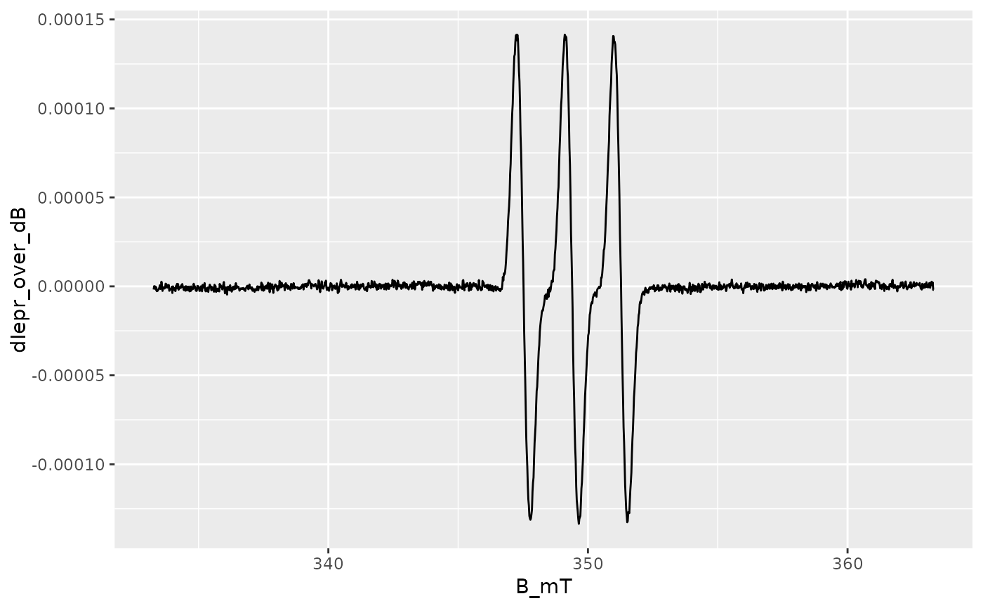
## simple `ggplot2` without any theme customization
ggplot2::ggplot(data = aminoxyl.data) +
ggplot2::geom_line(
ggplot2::aes(x = B_mT,y = dIepr_over_dB)
)
 #
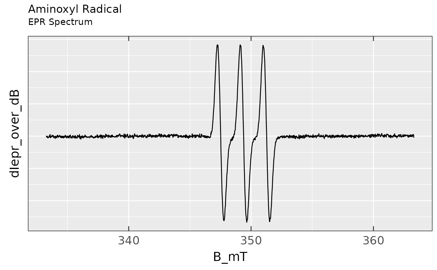
## simple `ggplot2` with `noY-ticks` theme and tile
## (+subtitle)
ggplot2::ggplot(data = aminoxyl.data) +
ggplot2::geom_line(
ggplot2::aes(x = B_mT,y = dIepr_over_dB)
) +
plot_theme_NoY_ticks() +
ggplot2::ggtitle(label = "Aminoxyl Radical",
subtitle = "EPR Spectrum")
#
## simple `ggplot2` with `noY-ticks` theme and tile
## (+subtitle)
ggplot2::ggplot(data = aminoxyl.data) +
ggplot2::geom_line(
ggplot2::aes(x = B_mT,y = dIepr_over_dB)
) +
plot_theme_NoY_ticks() +
ggplot2::ggtitle(label = "Aminoxyl Radical",
subtitle = "EPR Spectrum")
 #
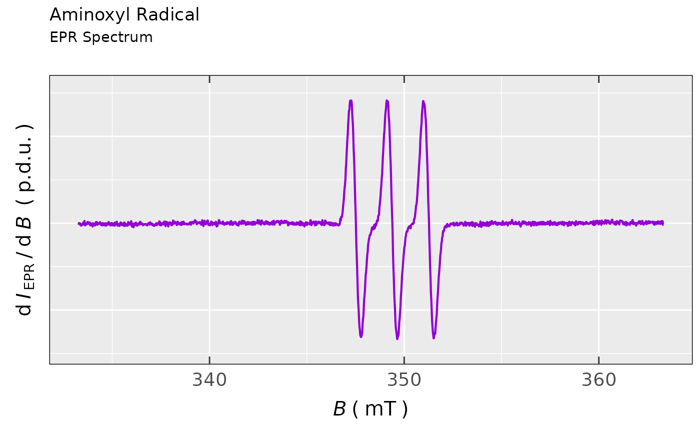
## comparison of EPR spectra generated
## by `plot_EPR_Specs()` and by the simple
## `ggplot2` with `noY-ticks` theme
plot_EPR_Specs(data.spectra = aminoxyl.data,
yTicks = FALSE) +
ggplot2::ggtitle(label = "Aminoxyl Radical",
subtitle = "EPR Spectrum")
#
## comparison of EPR spectra generated
## by `plot_EPR_Specs()` and by the simple
## `ggplot2` with `noY-ticks` theme
plot_EPR_Specs(data.spectra = aminoxyl.data,
yTicks = FALSE) +
ggplot2::ggtitle(label = "Aminoxyl Radical",
subtitle = "EPR Spectrum")
 #
## loading example data (incl. `Area` and `time`
## variables) from Xenon: decay of a triarylamine
## radical cation after its generation
## by electrochemical oxidation
triaryl_radCat_path <-
load_data_example(file =
"Triarylamine_radCat_decay_a.txt")
## corresponding data (double integrated EPR
## spectrum = `Area` vs `time`)
triaryl_radCat_data <-
readEPR_Exp_Specs(triaryl_radCat_path,
header = TRUE,
fill = TRUE,
select = c(3,7),
col.names = c("time_s","Area"),
x.unit = "s",
x.id = 1,
Intensity.id = 2,
qValue = 1700,
data.structure = "others") %>%
na.omit()
#
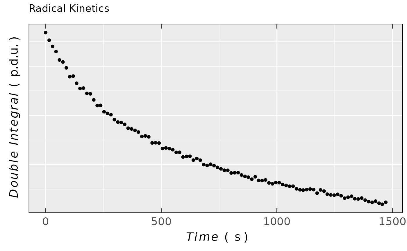
## simple plot of previous data using
## the `noY-ticks` theme
ggplot2::ggplot(data = triaryl_radCat_data) +
ggplot2::geom_point(
ggplot2::aes(x = time_s,y = Area)
) +
ggplot2::labs(title = "Radical Kinetics",
x = plot_labels_xyz(Time,s),
y = plot_labels_xyz(Double~~Integral,p.d.u.)) +
plot_theme_NoY_ticks()
#
## loading example data (incl. `Area` and `time`
## variables) from Xenon: decay of a triarylamine
## radical cation after its generation
## by electrochemical oxidation
triaryl_radCat_path <-
load_data_example(file =
"Triarylamine_radCat_decay_a.txt")
## corresponding data (double integrated EPR
## spectrum = `Area` vs `time`)
triaryl_radCat_data <-
readEPR_Exp_Specs(triaryl_radCat_path,
header = TRUE,
fill = TRUE,
select = c(3,7),
col.names = c("time_s","Area"),
x.unit = "s",
x.id = 1,
Intensity.id = 2,
qValue = 1700,
data.structure = "others") %>%
na.omit()
#
## simple plot of previous data using
## the `noY-ticks` theme
ggplot2::ggplot(data = triaryl_radCat_data) +
ggplot2::geom_point(
ggplot2::aes(x = time_s,y = Area)
) +
ggplot2::labs(title = "Radical Kinetics",
x = plot_labels_xyz(Time,s),
y = plot_labels_xyz(Double~~Integral,p.d.u.)) +
plot_theme_NoY_ticks()