General Ranking of Models/Fits by Concordance Correlation Coefficients and Plot

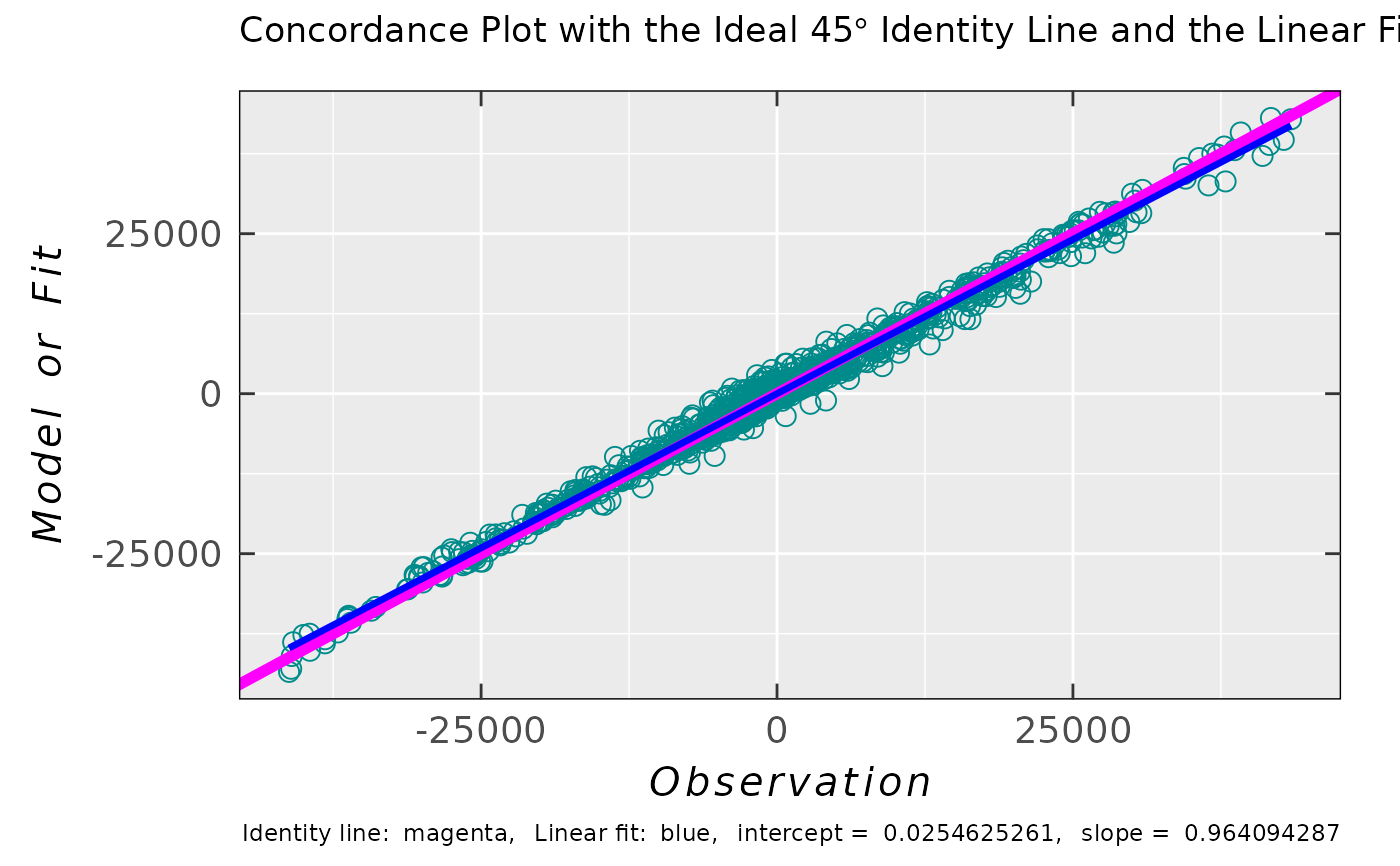
Evaluation of the robust and Lin's concordance correlation coefficients (CCCs). A correlation plot is provided with the $45\,\degree$ identity line as well as with the corresponding linear fit. Function can be applied as an agreement metric for the model/fit (y.vec) vs observation/experiment (x.vec, see e.g. eval_sim_EPR_isoFit). An optional original Bland-Altman plot is available if check.baplot = TRUE.

Usage

eval_CCC_forFit(x.vec, y.vec, check.baplot = FALSE)

Arguments

x.vec: Numeric vector (points), corresponding to any experiment or computation (observation), which is going to be compared to y.vec (i.e. its model/fit/simulation). For example this argument can be represented by the points (data frame column/vector) of an experimental EPR spectrum intensity to be fitted or simulated (can be returned by the eval_sim_EPR_isoFit using the Yourlist$ra$df$Experiment). In general, it can be applied to any vector of points/observations to be described by a suitable theoretical model/fit (see the y.vec argument).
y.vec: Numeric vector, equal to points of a model/fit of its corresponding x.vec counterpart. For example, this argument can be represented by points (data frame column/vector) of a simulated EPR intensity fit (can be returned by the eval_sim_EPR_isoFit using the Yourlist$ra$df$Simulation). In general, it can be applied to any model/fit which can reasonably describe the experimental or computational pattern of the x.vec.
check.baplot: Logical. If TRUE, the original Bland-Altman Plot can be presented as a Value list component. Default: check.baplot = FALSE.

Value

List with the following components:

df.ccc: Data frame object with four variables/columns and one row, summarizing the values of the robust CCC calculations as well as that of the Lin's one (see also Details and References). Each CCC value/column possess explanatory name (therefore it is compiled into df and not into named vector): "King's exponent $\delta$ = 1", "King's exponent $\delta$ = 1.5","King's exponent $\delta$ = 2 (Approaches Lin's CCC)" and finally "Lin's CCC".
plot.cc: Ggplot2 object function, built to visualize the correlation of both original vectors (y.vec vs x.vec). In ideal case all data points are perfectly aligned with the $45\,\degree$ identity/concordance line (with the intercept 0 and the slope 1). In addition, a linear fit is presented for a comparison to identity line. Function controls appearence of the plot: color, size, shape, linewidth and linetype of points and the two lines, separately. See also point and line aesthetics of the {ggplot2} package.
Cb: Numeric value of Lin's CCC bias-correction factor (accuracy), which measures how far the linear fit line deviates from the $45\,\degree$ identity line. No deviation occurs when Cb = 1. In general, Cb $\leq$ 1, where Cb = Lin's CCC / r, with the r corresponding to Pearson's correlation coefficient.
baplot: If check.baplot = FALSE (default), baplot = NULL. Otherwise, original (non-robust) Bland-Altman plot is displayed, as a {ggplot2} object, and detects the presence of any systematic bias as well as possible outliers between x.vec and y.vec. It actually shows the paired Difference (with $95\,\%$ confidence band - the light blue area also known as limits of agreement) vs corresponding paired Mean value of those two vectors.

Details

Correlation between the two continuous random variables (bivariate correlation) is used to analyze their linear relationship and the most common measure of such correlation/association is expressed by the Pearson's correlation coefficient (CC). However, when it comes to agreement between the experiment/observation and its corresponding model/fit (e.g. simulation fit of an experimental EPR spectrum) usually one has to consider not only the qualitative aspect (EPR spectrum shape similarity) of agreement but also the quantitative one (i.e. the EPR spectrum intensity). In addition, the Pearson's CC can be sensitive to outliers and skewness of the variable(s) distribution. Therefore, a more robust agreement indices were introduced (see below and Valleyos RO (2026) and King TS, Chinchilli VM (2001) in the References.)

The evaluation is based on the widely recognized CCC, developed by Lin (see Lin LIK (1989) in the References), which, while sharing certain properties with the Pearson correlation coefficient (wide infra), provides a more appropriate measure of deviation from the $45\,\degree$ line passing through the origin (with the intercept = 0 and the slope = 1). This is due to the fact that the CCC accounts for both the magnitude and direction of the deviation from the 45-degree line in the graphical representation of an agreement. The Lin's CCC is denoted as $\hat{\rho}_c$ (see also Value and df.ccc). It can be expressed in the following form: $$\hat{\rho}_c = 2\,S_{XY}^{}\,/\,(S_X^2 + S_Y^2 + (\bar{X} - \bar{Y})^2)$$ where $S_{XY}^{} = (1/n)\,\sum_{i=1}^n (X_i - \bar{X})(Y_i - \bar{Y})$, $S_X^2 = (1/n)\,\sum_{i=1}^n (X_i - \bar{X})^2$ and similarly $S_Y^2 = (1/n)\,\sum_{i=1}^n (Y_i - \bar{Y})^2$. $\bar{X}$ and $\bar{Y}$ correspond to mean values of the variables/vectors (refer to the arguments x.vec and y.vec). The Lin's CCC ($\hat{\rho}_c$) can be also calculated taking into account the Pearson coefficient $r$: $$\hat{\rho}_c = r\,Cb$$ where $Cb = 2\,/\,(v + (1/v) + u^2)$ with $v = S_X^{}\,/\,S_Y^{}$ and $u = (\bar{X} - \bar{Y})\,/\,\sqrt{S_X^{}\,S_Y^{}}$ ($S_X^{} = \sqrt{S_X^2}$ and $S_Y^{} = \sqrt{S_Y^2}$) denoting as a scale and location shifts, respectively. The $Cb$ is the correction factor, showing how the linear fit of y.vec ($Y$) vs x.vec ($X$) deviates from the $45\,\degree$ identity line. Because the Lin's CCC ($\hat{\rho}_c$) contains squared distances from the mean values, it can be sensitive to outliers in the Model/Fit vs Observations (or in the residual analysis).

In order to "robustify" the Lin's CCC, King, Chinchilli and Valleyos (see articles in the References) suggested a general distance function $g(z) = |z|^{\delta}$ where the Monte Carlo simulations indicated that the best performing $\delta$ (in terms of robustness) are $\delta = 1$ and $\delta = 1.5$ (with $\delta = 2$ approaching the original Lin's CCC). Such concordance correlation coefficient can be expressed as follows (proposed by Valleyos RO (2026) see References): $$\hat{\rho} = 1 - ((1/n)\,\sum_{i=1}^n |X_i - Y_i|^{\delta})\,/\,((1/n^2)\,\sum_{i=1}^n\sum_{j=1}^n |X_i - Y_j|^{\delta})$$ The denominator is the mean distance ($g(z)$) across the all $X,Y$ matrix elements (expectation under independence); the numerator is the mean distance over matched pairs. Setting $\delta = 2$ recovers the Lin's CCC; $\delta = 1$ gives the robust, outlier-resistant version. The cross pairs are calculated using outer and the coefficients are evaluated for all three $\delta = 1$, $\delta = 1.5$ and $\delta = 2$. McBride GB (2005) (see the References) suggested the following descriptive scale for values of the concordance correlation coefficient (for continuous variables):

CCC Value	Strength of Agreement
$< 0.90$	Poor
$0.90 - 0.95$	Moderate
$0.95 - 0.99$	Substantial
$> 0.99$	Almost perfect

References

Valleyos RO (2026). "Agreement Coefficients for Continuous Variables: A Review", Environmetric, 37(6), e70117-19, https://onlinelibrary.wiley.com/doi/10.1002/env.70117.

King TS, Chinchilli VM (2001). "Robust Estimators of the Concordance Correlation Coefficient", J. Biopharm. Stat., 11(3), 83-105, https://www.tandfonline.com/doi/full/10.1081/BIP-100107651.

Lin LIK (1989). "A Concordance Correlation Coefficient to Evaluate Reproducibility", Biometrics, 45(1), 255-268, https://www.jstor.org/stable/2532051.

McBride GB (2005) "A proposal for strength-of-agreement criteria for Lin's Concordance Correlation Coefficient", NIWA Client Report: HAM2005-062, https://www.medcalc.org/en/download/pdf/McBride2005.pdf.

Oliveira TP, Moral RA, Zocchi SS, Demetrio CGB, Hinde J. (2020). "lcc: an R package to estimate the concordance correlation, Pearson correlation and accuracy over time", PeerJ, 8, e9850-29, https://doi.org/10.7717/peerj.9850.

Svetunkov I (2022). Statistics for Business Analytics, Version 2025, https://openforecast.org/sba/.

Bulut H, Zobu M, Saglam V (2026). "A High-Breakdown MCD-Based Robust Concordance Correlation Coefficient", Mathematics, 14(1), 196-22, https://doi.org/10.3390/math14010196.

Nguyen M (2020). "A Guide on Data Analysis", https://bookdown.org/mike/data_analysis/.

James G, Witten D, Hastie T, Tibshirani R (2021). An Introduction to Statistical Learning: with Applications in R, 2nd edition, Springer, ISBN 978-1-071-61417-4, https://www.statlearning.com/.

Karun MK, Puranik A (2021). "BA.plot: An R function for Bland-Altman Analysis", Clin. Epidemiol. Glob. Health, 12,100831-3, https://doi.org/10.1016/j.cegh.2021.100831.

Examples

## load experimental TMPD radical cation
## EPR data/spectrum
data.file.path <-
  load_data_example(file =
    "TMPD_specelchem_accu_b.asc")
data.tmpd.expr <-
  readEPR_Exp_Specs(
    path_to_file = data.file.path,
    col.names = c("B_G","dIepr_over_dB"),
    qValue = 3500,
    origin = "winepr"
   )
#
## simulation fit for TMPD radical cation
sim.fit.tmpd.spec <- eval_sim_EPR_isoFit(
  data.spectr.expr = data.tmpd.expr,
  nu.GHz = 9.814155,
  nuclear.system.noA = list(
    list("14N", 2),
    list("1H", 4),
    list("1H", 12)
  ),
  lineG.content = 0.42,
  baseline.correct = "constant",
  optim.method = "neldermead",
  optim.params.init = c(
    2.00304,
    0.52, 0.51,
    0,
    3.2e5,
    19.62, 5.49, 19.54
  ),
  Nmax.evals = 64,
  Blim = c(3450,3550),
  check.fit.plot = TRUE
)
#> 
#> 
 EPR simulation parameters are currently being optimized by   NELDERMEAD ;  method   1   of   1 ... 
#> 
#> 
 Done!  ( 100  %)    elapsed time  6.7  s 
#
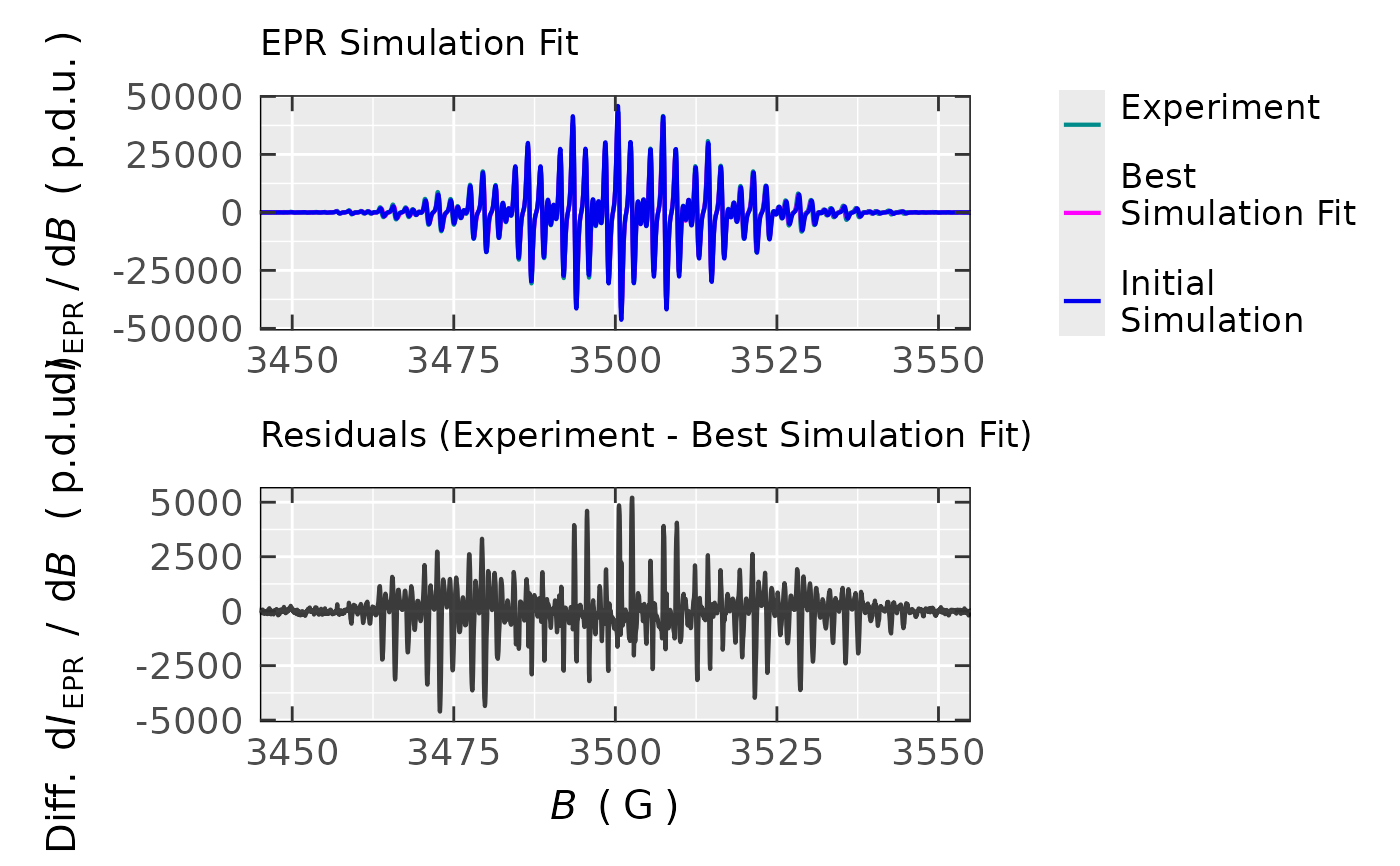
## EPR spectra comparison
sim.fit.tmpd.spec$plot

#
## experiment + simulation fit concordance
concord.list <- eval_CCC_forFit(
  x.vec =
    sim.fit.tmpd.spec$ra$df$Experiment,
  y.vec =
    sim.fit.tmpd.spec$ra$df$Simulation
)
#
## concordance coefficients (CC)
concord.list$df.ccc
#>   King's exponent δ = 1 King's exponent δ = 1.5
#> 1           0.924784383             0.978864734
#>   King's exponent δ = 2 (Approaches Lin's CCC)   Lin's CCC
#> 1                                  0.993814035 0.993814035
#
## plot
concord.list$plot.cc(point.shape = 1)

#
## accuracy (related to Lin's CCC)
concord.list$Cb
#> [1] 0.999524747
#
## Pearson correlation via Lin's CCC and Cb
concord.list$df[1,4] / concord.list$Cb
#> [1] 0.994286572
#
## Pearson correlations by `cor()`
## function for comparison
sim.fit.tmpd.spec$cor.df()
#>             Experiment  Simulation   Residuals
#> Experiment 1.000000000 0.994286572 0.327746170
#> Simulation 0.994286572 1.000000000 0.225025836
#> Residuals  0.327746170 0.225025836 1.000000000

CCC Value	Strength of Agreement
\(< 0.90\)	Poor
\(0.90 - 0.95\)	Moderate
\(0.95 - 0.99\)	Substantial
\(> 0.99\)	Almost perfect